Feature #1205

Improve computational speed for CTA binned analysis
| Status: | Closed | Start date: | ||
|---|---|---|---|---|
| Priority: | Urgent | Due date: | 12/19/2014 | |
| Assigned To: |  Knödlseder Jürgen Knödlseder Jürgen | % Done: | 100% | |
| Category: | - | |||
| Target version: | 1.0.0 | |||
| Duration: |
Description
As the ctools are more and more used for science simulations, a speed-up of the binned analysis seems now urgently required.
devel-20140721.png (53.9 KB)
git-GSkymap-cache.png (61.2 KB)
git-ptsrc-cache.png (63.5 KB)
git-no-dyn.png (101 KB)

Recurrence
No recurrence.
History
#1
 Updated by Knödlseder Jürgen over 10 years ago
- Description updated (diff)
- Priority changed from Normal to Urgent
#2
Updated by Knödlseder Jürgen over 10 years ago
- Target version set to 1.0.0
#3
Updated by Knödlseder Jürgen over 10 years ago
- Due date set to 12/19/2014
#4
Updated by Knödlseder Jürgen over 10 years ago
- Status changed from New to In Progress
- Assigned To set to Knödlseder Jürgen
Start now to tackle that one.
#5
Updated by Knödlseder Jürgen over 10 years ago
Here an initial timing analysis using the script example_binned_ml_fit.py. Cube-style is a factor of 2 slower than standard binned analysis, possibly due to the skymap interpolation when accessing exposure cube and PSF cube information. This can be optimized.
+===============================================+
| Binned maximum likelihood fitting of CTA data |
+===============================================+
=== GOptimizerLM ===
 Optimized function value ..: 18210.806
 Absolute precision ........: 1e-06
 Optimization status .......: converged
 Number of parameters ......: 11
 Number of free parameters .: 5
 Number of iterations ......: 3
 Lambda ....................: 1e-06
=== GOptimizerLM ===
 Optimized function value ..: 21582.340
 Absolute precision ........: 1e-06
 Optimization status .......: converged
 Number of parameters ......: 5
 Number of free parameters .: 3
 Number of iterations ......: 8
 Lambda ....................: 1e-11
 Test statistics ...........: 6743.068
 Elapsed time ..............: 10.560 sec

+===================================================+
| Cube-style maximum likelihood fitting of CTA data |
+===================================================+
=== GOptimizerLM ===
 Optimized function value ..: 18278.402
 Absolute precision ........: 1e-06
 Optimization status .......: converged
 Number of parameters ......: 11
 Number of free parameters .: 5
 Number of iterations ......: 4
 Lambda ....................: 1e-07
=== GOptimizerLM ===
 Optimized function value ..: 21582.340
 Absolute precision ........: 1e-06
 Optimization status .......: converged
 Number of parameters ......: 5
 Number of free parameters .: 3
 Number of iterations ......: 9
 Lambda ....................: 1e-12
 Test statistics ...........: 6607.875
 Elapsed time ..............: 21.870 sec
#6
Updated by Knödlseder Jürgen over 10 years ago
After adding a pre-computation cache to the GSkymap interpolation operator, the following results were obtained. The cube-style analysis went done from 21.87 sec to 9.54 sec and is now comparable to the conventional binned analysis. The drawback of the skymap computations were substantially reduced.
+===============================================+
| Binned maximum likelihood fitting of CTA data |
+===============================================+
=== GOptimizerLM ===
 Optimized function value ..: 18210.806
 Absolute precision ........: 1e-06
 Optimization status .......: converged
 Number of parameters ......: 11
 Number of free parameters .: 5
 Number of iterations ......: 3
 Lambda ....................: 1e-06
=== GOptimizerLM ===
 Optimized function value ..: 21582.340
 Absolute precision ........: 1e-06
 Optimization status .......: converged
 Number of parameters ......: 5
 Number of free parameters .: 3
 Number of iterations ......: 8
 Lambda ....................: 1e-11
 Test statistics ...........: 6743.068
 Elapsed time ..............: 11.179 sec

+===================================================+
| Cube-style maximum likelihood fitting of CTA data |
+===================================================+
=== GOptimizerLM ===
 Optimized function value ..: 18396.601
 Absolute precision ........: 1e-06
 Optimization status .......: converged
 Number of parameters ......: 11
 Number of free parameters .: 5
 Number of iterations ......: 4
 Lambda ....................: 1e-07
=== GOptimizerLM ===
 Optimized function value ..: 21582.340
 Absolute precision ........: 1e-06
 Optimization status .......: converged
 Number of parameters ......: 5
 Number of free parameters .: 3
 Number of iterations ......: 9
 Lambda ....................: 1e-12
 Test statistics ...........: 6371.478
 Elapsed time ..............: 9.538 sec
#7
Updated by Knödlseder Jürgen over 10 years ago
I implemented caching classes GCTASourceCube and GCTASourceCubePointSource that are caching the effective area, the distance between spatial pixels and the source direction (Delta cache), as well as the PSF values for the specific source direction and the energies in the event cube (branch: 1205-improve-binned-analysis).
- Effective area cache: 9.0 ⇒ 9.0 (no difference)
- Delta cache: 9.4 ⇒ 9.2 sec (3% improvement)
- PSF cache: 9.0 ⇒ 9.2 sec (using the cache makes things slower)
The conclusion is that all the caching of response values does not bring a speed increase. Interpolating directly in the exposure and PSF cubes is pretty fast. The only slight speed difference comes from caching the distances between source position and bin centre.
#8
Updated by Knödlseder Jürgen over 10 years ago
- % Done changed from 0 to 10
#9
Updated by Knödlseder Jürgen over 10 years ago
Next thing to test: improved caching of the spectral component.
#10
Updated by Knödlseder Jürgen over 10 years ago
Adding full caching to GModelSpectralPlaw brings slight speed improvement. Full caching means that also value and gradients are only computed when the energy or some parameters change.
+===============================================+
| Binned maximum likelihood fitting of CTA data |
+===============================================+
=== GOptimizerLM ===
 Optimized function value ..: 18210.806
 Absolute precision ........: 1e-06
 Optimization status .......: converged
 Number of parameters ......: 11
 Number of free parameters .: 5
 Number of iterations ......: 3
 Lambda ....................: 1e-06
=== GOptimizerLM ===
 Optimized function value ..: 21582.340
 Absolute precision ........: 1e-06
 Optimization status .......: converged
 Number of parameters ......: 5
 Number of free parameters .: 3
 Number of iterations ......: 8
 Lambda ....................: 1e-11
 Test statistics ...........: 6743.068
 Elapsed time ..............: 10.083 sec

+===================================================+
| Cube-style maximum likelihood fitting of CTA data |
+===================================================+
=== GOptimizerLM ===
 Optimized function value ..: 18396.601
 Absolute precision ........: 1e-06
 Optimization status .......: converged
 Number of parameters ......: 11
 Number of free parameters .: 5
 Number of iterations ......: 4
 Lambda ....................: 1e-07
=== GOptimizerLM ===
 Optimized function value ..: 21582.340
 Absolute precision ........: 1e-06
 Optimization status .......: converged
 Number of parameters ......: 5
 Number of free parameters .: 3
 Number of iterations ......: 9
 Lambda ....................: 1e-12
 Test statistics ...........: 6371.478
 Elapsed time ..............: 8.947 sec
#11
Updated by Knödlseder Jürgen over 10 years ago
- % Done changed from 10 to 20
Not sure if at the end very much can be gained. Now needs a kachgrind investigation to understand better where the bottle necks are.
#12
Updated by Knödlseder Jürgen over 10 years ago
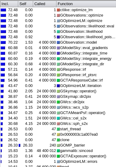
- File devel-20140721.png added
Attached a valgrind analysis of the current (21/07/2014) devel branch displayed by Kcachegrind. A substantial amount of the time (42%) is spent in the GSkymap::operator() which is used in GCTAResponseCube::irf for exposure and PSF cube access. Note that in this version, no GSkymap::operator() cache had been implemented. Note also that a substantial amount of time is spent in the GOMP_barrier, which is related to OpenMP parallel processing (not clear why this is an issue here).

#13
Updated by Knödlseder Jürgen over 10 years ago
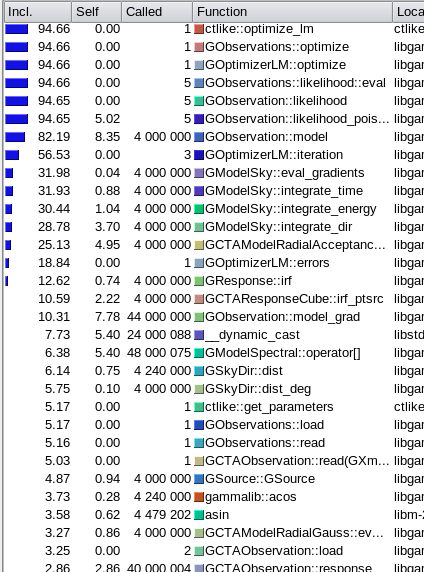
- File git-GSkymap-cache.png added
GSkymap::operator(). Now the time is essentially spent in GObservation::model, from which
- 35% goes to
GModelRadialAcceptance::eval_gradients() - 15% goes to
GObservation::model_grad - 50% goes to
GModelSky::eval_gradients()
Interestingly, the background model computation (35%) takes not much less time than the sky model computation (50%). For some reason I do not understand, GOMP_barrier does not longer show up.
#14
Updated by Knödlseder Jürgen over 10 years ago
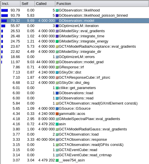
- File git-ptsrc-cache.png added
- 37% goes to GModelRadialAcceptance::eval_gradients()
- 15% goes to GObservation::model_grad
- 47% goes to GModelSky::eval_gradients()
GObservation::model(8.4%, 4 000 000 calls)GObservation::model_grad(7.8%, 44 000 000 calls)__dynamic_cast(5.4%, 24 000 088 calls) (we definitely do this too often, for security reasons; there are already 4% of this inGCTAResponseCube::irf_ptsrc)GModelSpectral::operator[](5.4%, 48 000 075 calls)GCTAModelRadialAcceptance::eval_gradients(5%, 4 000 000 calls)GCTAObservation::response()(2.9%, 40 000 004 calls) (not clear why this needs time, there is just a pointer is NULL check)GModelSpectral::size(1.6%, 80 000 100 calls) (not clear why this takes time, maybe called too often? method could be inlined)
Globally, however, the code looks quite well equilibrated between the various functions.

#15
Updated by Knödlseder Jürgen over 10 years ago
- % Done changed from 20 to 30
Here the result after replacing some dynamic_cast by static_cast or GClassCode types, and after removing unnecessary range checks on spatial, spectral and temporal model indices. This led to some 10% speed improvement. Nothing really dramatic.
+===============================================+
| Binned maximum likelihood fitting of CTA data |
+===============================================+
=== GOptimizerLM ===
 Optimized function value ..: 18210.806
 Absolute precision ........: 1e-06
 Optimization status .......: converged
 Number of parameters ......: 11
 Number of free parameters .: 5
 Number of iterations ......: 3
 Lambda ....................: 1e-06
=== GOptimizerLM ===
 Optimized function value ..: 21582.340
 Absolute precision ........: 1e-06
 Optimization status .......: converged
 Number of parameters ......: 5
 Number of free parameters .: 3
 Number of iterations ......: 8
 Lambda ....................: 1e-11
 Test statistics ...........: 6743.068
 Elapsed time ..............: 9.396 sec

+===================================================+
| Cube-style maximum likelihood fitting of CTA data |
+===================================================+
=== GOptimizerLM ===
 Optimized function value ..: 18396.601
 Absolute precision ........: 1e-06
 Optimization status .......: converged
 Number of parameters ......: 11
 Number of free parameters .: 5
 Number of iterations ......: 4
 Lambda ....................: 1e-07
=== GOptimizerLM ===
 Optimized function value ..: 21582.340
 Absolute precision ........: 1e-06
 Optimization status .......: converged
 Number of parameters ......: 5
 Number of free parameters .: 3
 Number of iterations ......: 9
 Lambda ....................: 1e-12
 Test statistics ...........: 6371.478
 Elapsed time ..............: 8.069 sec
#16
Updated by Knödlseder Jürgen over 10 years ago
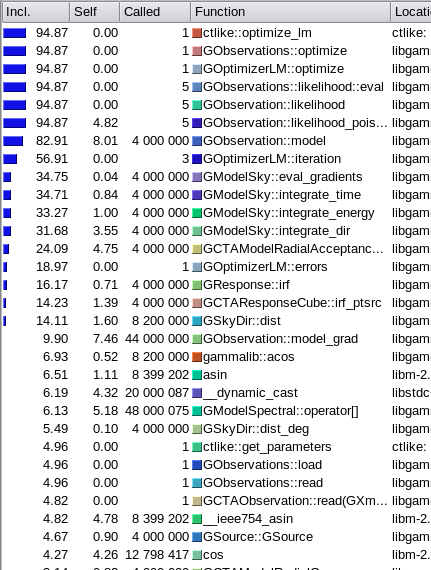
- File git-no-dyn.png added
GObseration::modeltakes a considerable amount of time (10%), not sure why ... (the method is basically doing bookkeeping)GCTAResponseCube::irf_ptsrctakes less than 2% of the time, response computation is really not an issueGObservation::model_gradtakes also 9%, this is the price for fitting the background model shape

#17
Updated by Knödlseder Jürgen over 10 years ago
- % Done changed from 30 to 40
I worked on improving the GObservation::model and GObservation::model_grad computation. This gave a little speed increase
+===============================================+
| Binned maximum likelihood fitting of CTA data |
+===============================================+
=== GOptimizerLM ===
 Optimized function value ..: 18210.806
 Absolute precision ........: 1e-06
 Optimization status .......: converged
 Number of parameters ......: 11
 Number of free parameters .: 5
 Number of iterations ......: 3
 Lambda ....................: 1e-06
=== GOptimizerLM ===
 Optimized function value ..: 21582.340
 Absolute precision ........: 1e-06
 Optimization status .......: converged
 Number of parameters ......: 5
 Number of free parameters .: 3
 Number of iterations ......: 8
 Lambda ....................: 1e-11
 Test statistics ...........: 6743.068
 Elapsed time ..............: 10.428 sec

+===================================================+
| Cube-style maximum likelihood fitting of CTA data |
+===================================================+
=== GOptimizerLM ===
 Optimized function value ..: 18396.601
 Absolute precision ........: 1e-06
 Optimization status .......: converged
 Number of parameters ......: 11
 Number of free parameters .: 5
 Number of iterations ......: 4
 Lambda ....................: 1e-07
=== GOptimizerLM ===
 Optimized function value ..: 21582.340
 Absolute precision ........: 1e-06
 Optimization status .......: converged
 Number of parameters ......: 5
 Number of free parameters .: 3
 Number of iterations ......: 9
 Lambda ....................: 1e-12
 Test statistics ...........: 6371.478
 Elapsed time ..............: 7.885 sec
#18
Updated by Knödlseder Jürgen over 10 years ago
The former tests took more iterations for the cube-style analysis than for the standard binned analysis. This has now been changed by improving the precision of the PSF cube in the test data. The logL of the cube-style analysis is now much closer to that of the binned analysis, and cube-style is about 50% faster.
+===============================================+
| Binned maximum likelihood fitting of CTA data |
+===============================================+
=== GOptimizerLM ===
 Optimized function value ..: 18210.806
 Absolute precision ........: 1e-06
 Optimization status .......: converged
 Number of parameters ......: 11
 Number of free parameters .: 5
 Number of iterations ......: 3
 Lambda ....................: 1e-06
=== GOptimizerLM ===
 Optimized function value ..: 21582.340
 Absolute precision ........: 1e-06
 Optimization status .......: converged
 Number of parameters ......: 5
 Number of free parameters .: 3
 Number of iterations ......: 8
 Lambda ....................: 1e-11
 Test statistics ...........: 6743.068
 Elapsed time ..............: 9.816 sec

+===================================================+
| Cube-style maximum likelihood fitting of CTA data |
+===================================================+
=== GOptimizerLM ===
 Optimized function value ..: 18212.501
 Absolute precision ........: 1e-06
 Optimization status .......: converged
 Number of parameters ......: 11
 Number of free parameters .: 5
 Number of iterations ......: 3
 Lambda ....................: 1e-06
=== GOptimizerLM ===
 Optimized function value ..: 21582.340
 Absolute precision ........: 1e-06
 Optimization status .......: converged
 Number of parameters ......: 5
 Number of free parameters .: 3
 Number of iterations ......: 8
 Lambda ....................: 1e-11
 Test statistics ...........: 6739.677
 Elapsed time ..............: 6.793 sec
#19
Updated by Knödlseder Jürgen over 10 years ago
Consider the point source analysis as optimized. Hardly see any opportunity to do much better. Now will tackle extended sources and diffuse emission.
#20
Updated by Knödlseder Jürgen over 10 years ago
- Status changed from In Progress to Closed
- % Done changed from 40 to 100
Seems to be as fast as possible for now. Not excluded that improvement can still be made, but at least a considerable effort has been invested in making things faster.