Action #2403

Check if the energy dispersion integration can be optimised
| Status: | Closed | Start date: | 03/08/2018 | |
|---|---|---|---|---|
| Priority: | Normal | Due date: | ||
| Assigned To: |  Knödlseder Jürgen Knödlseder Jürgen | % Done: | 100% | |
| Category: | - | |||
| Target version: | 1.5.1 | |||
| Duration: |
Description
Try to see whether we can reduce the integration precision for the energy dispersion without loosing accuracy in the analysis.
The integration precision is set in GResponse::convolve (constant iter).
South_z20_average_50h_v1.5.1.png (57.6 KB)
South_z20_average_50h_v1.5.0.png (70 KB)
South_z20_average_50h_kludge5s.png (64.5 KB)
South_z20_average_50h_kludge10s.png (64.5 KB)
South_z20_average_50h_kludge3s5s.png (59.6 KB)
South_z20_average_50h_offset0.png (185 KB)
South_z20_average_50h_offset0_try1.png (195 KB)


Recurrence
No recurrence.
History
#1
 Updated by Knödlseder Jürgen about 7 years ago
- File South_z20_average_50h_v1.5.1.png added
- Status changed from New to In Progress
- % Done changed from 0 to 10
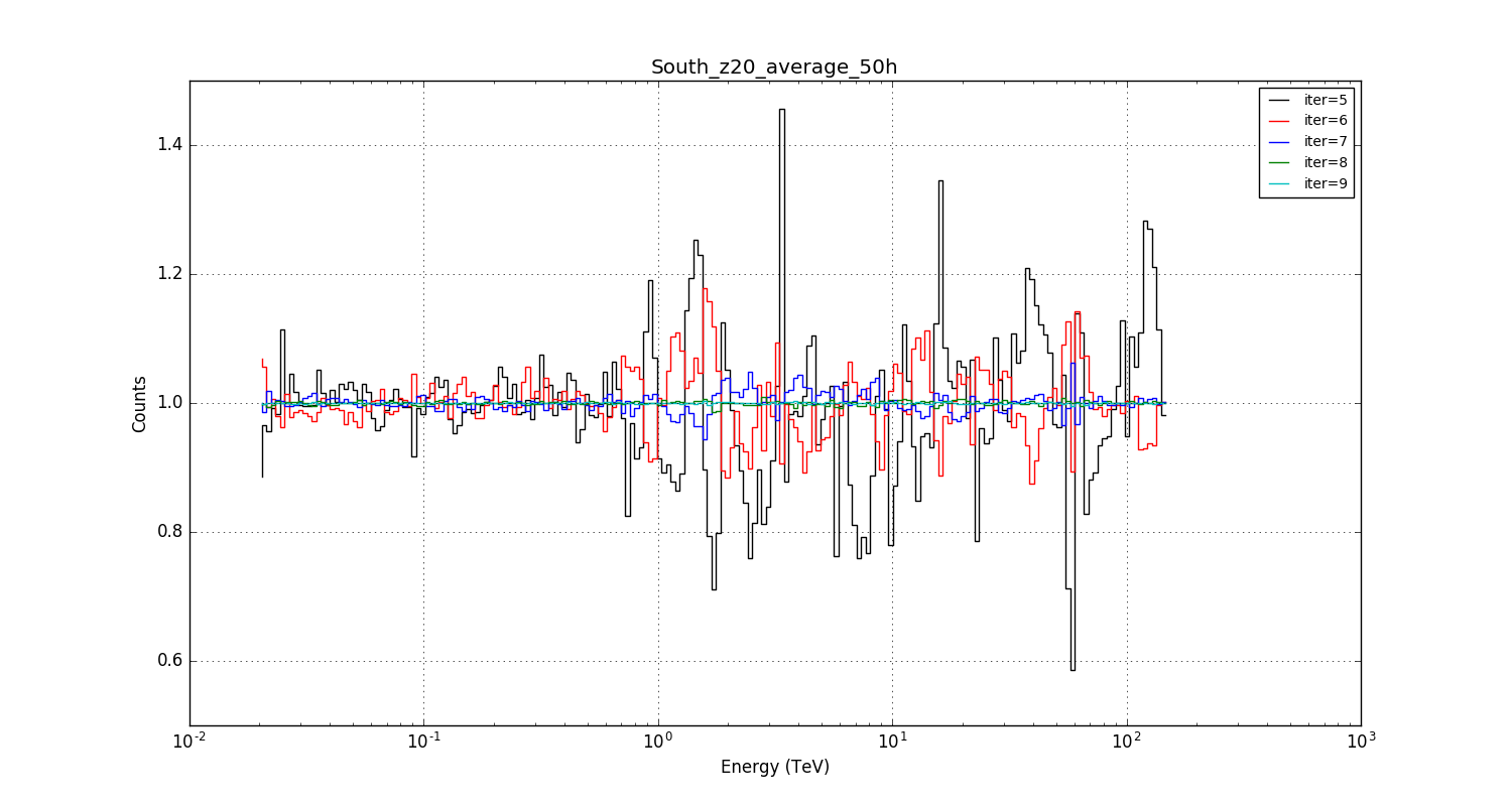
I had actually not recognised how bad the situation really is. Below a plot for the current kludge implementation (clipping and slight smooth in etrue) where I changed the number of integration steps using the iter parameter (recall: iter is the fixed number of iterations in a Romberg integration). The plot shows the fractional difference in the model computation as function of energy with respect to a very high precision computation done with iter=10.
The current value that is used is iter=6 (red line), and it turns out that for that value there are spikes that reach about 15% of the reference value. Only for iter>=8 the integration converges, and uncertainties are at the level of a few percent.

#2
Updated by Knödlseder Jürgen about 7 years ago
- File South_z20_average_50h_v1.5.0.png added
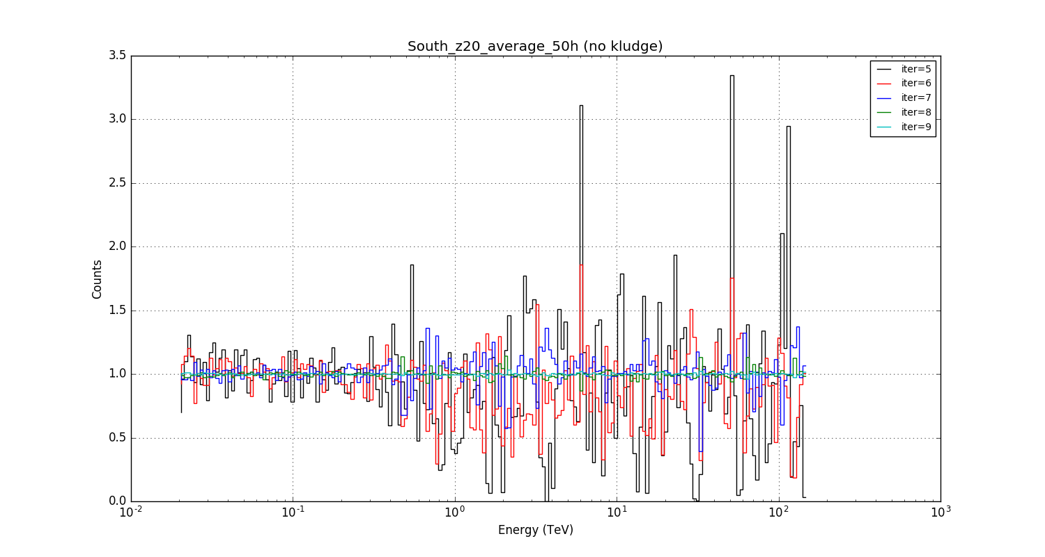
Just to illustrate how bad it was before: at least the kludge goes in the right direction.
#3
Updated by Knödlseder Jürgen about 7 years ago
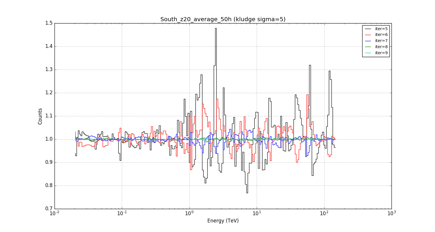
- File South_z20_average_50h_kludge5s.png added
A 5 sigma smoothing in true energy instead of a 3 sigma smoothing does not really change the picture.
#4
Updated by Knödlseder Jürgen about 7 years ago
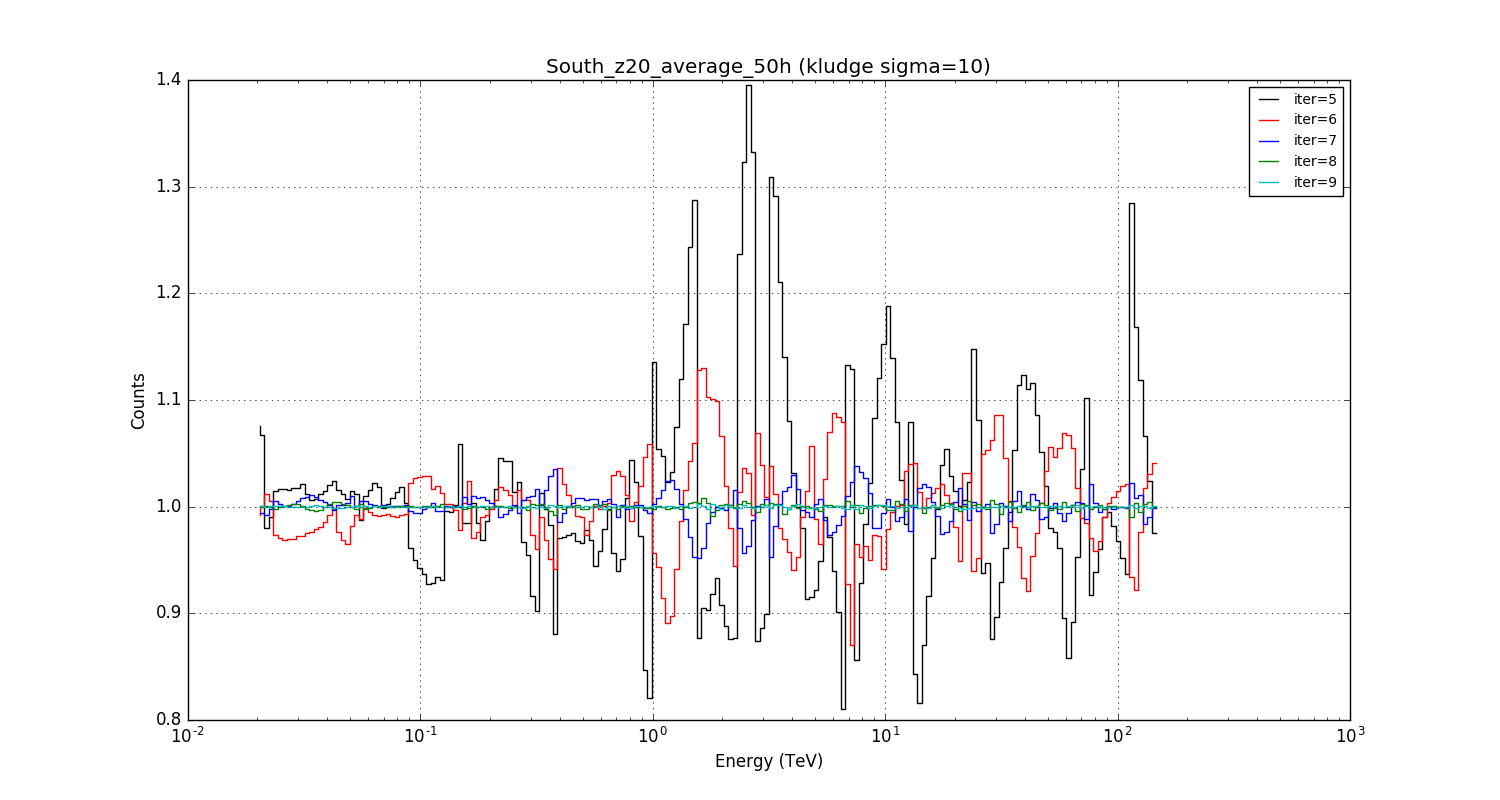
- File South_z20_average_50h_kludge10s.png added
Going to a smoothing sigma of 10 pixels in etrue improves the situation as expected, but the accuracy with iter=6 is still not better than about 10% at high energies.
#5
Updated by Knödlseder Jürgen about 7 years ago
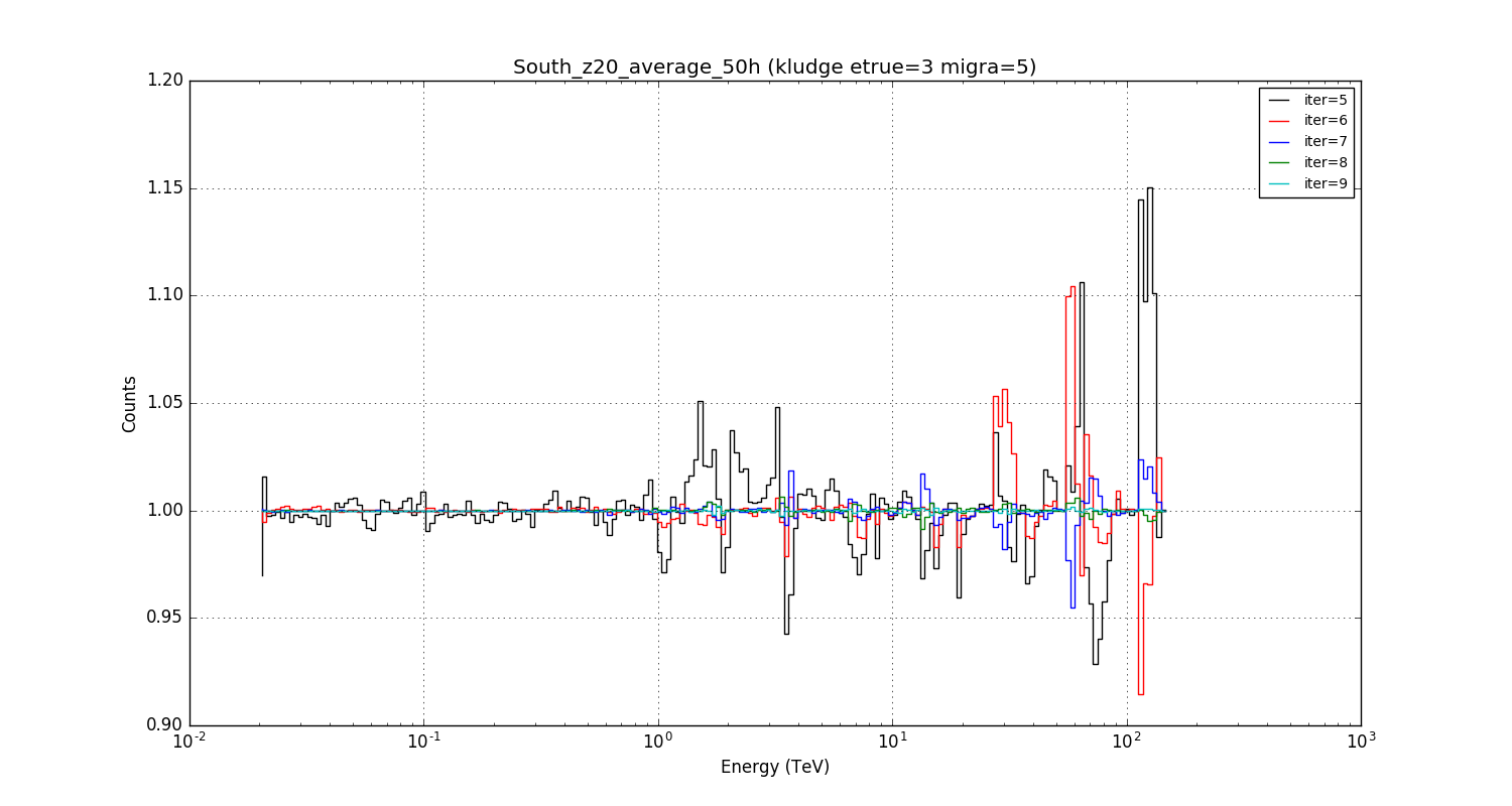
- File South_z20_average_50h_kludge3s5s.png added
Smoothing bin 3 bins in etrue and 5 bins in migra improves the situation. The migra smoothing obviously has a strong impact on the required integration precision. This is certainly the way to follow. The biggest residuals are at the highest energies, where the statistic is lowest in the migration matrix.
#6
Updated by Knödlseder Jürgen about 7 years ago
- File South_z20_average_50h_offset0.png added
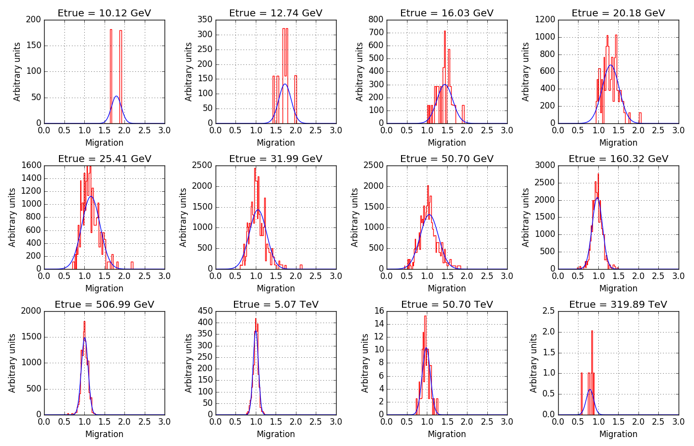
The following figure illustrates the issue with the energy dispersion matrix. The noise in a given true energy bin is considerable, even for the domain where the statistic is high.

#7
Updated by Knödlseder Jürgen about 7 years ago
- File South_z20_average_50h_offset0_try1.png added
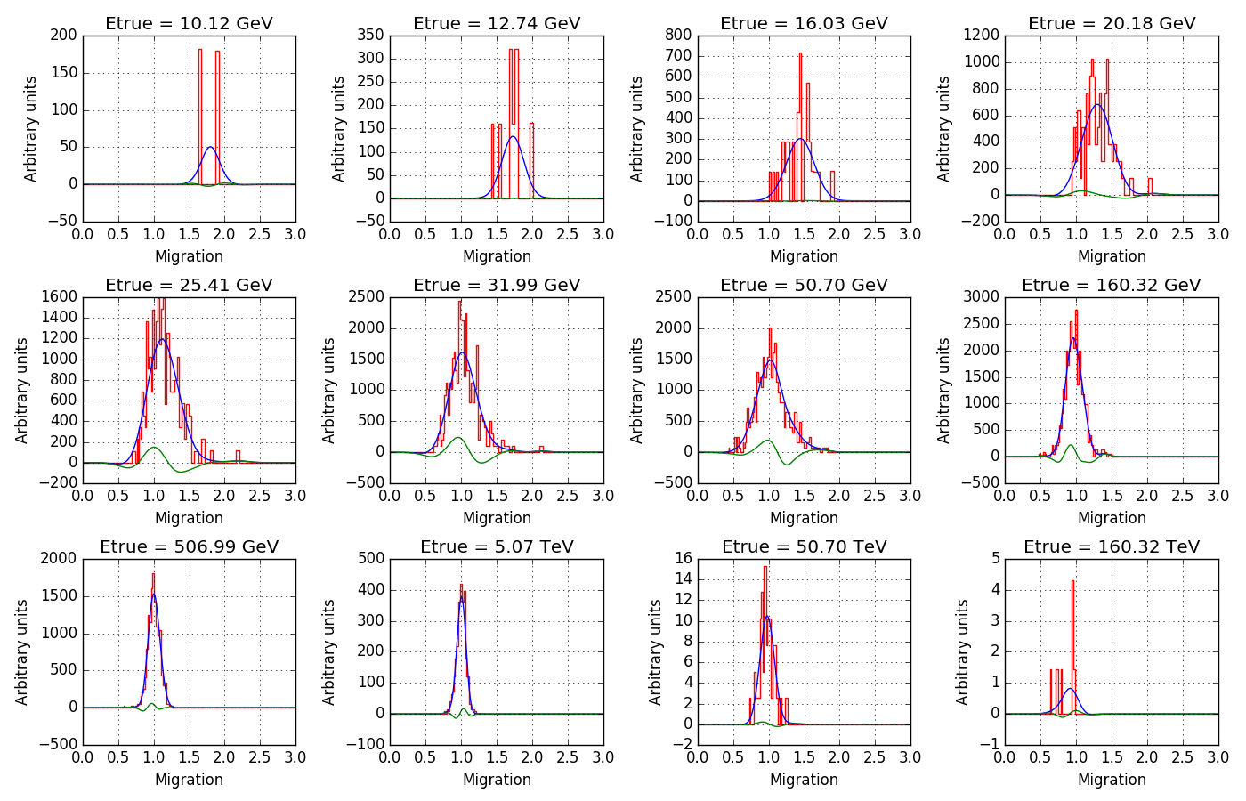
Here an attempt to get rid of the noise (blue curves).
The algorithm first determines for each true energy bin the mean and rms migration value since the zero order shape of the energy migration is a Gaussian (that’s in fact the blue curve shown in the plot above). The Gaussian is then subtracted from the migration values and the residual is then smoothed by a Gaussian with a certain width, and the smoothed residual is then added back to the Gaussian. In the plot below, the smoothed residual is shown as green line.
The trick now is to change the Gaussian smoothing sigma as function of the noise. For that purpose, the mean number of events per filled migration pixel mean is determined. This is hampered by the fact that the migration values have been rescaled, but by assuming that the minimum non-zero pixel value corresponds to one event one can get an estimate of the mean number of events per filled pixel.
Then the number of pixels num_pixels that are covered by the migration values is computed, computing the difference between the last and first non-zero migration pixels. To handle the case of a single filled pixel, we assume that at least 10% of the migration pixels are covered by the migration matrix.
Finally, the sigma (in number of pixels) is computed using
sigma = 0.5 * num_pixels / mean
This is an empiric scaling law that is proportional to the number of pixels covered and inversely proportional to the estimated mean number of counts in a pixel.

#8
Updated by Knödlseder Jürgen almost 7 years ago
- Status changed from In Progress to Closed
- % Done changed from 10 to 100
It turned out that the current level of integration is needed to give accurate results.