Bug #2458
Extended model fits better than diffuse map
| Status: | Closed | Start date: | 04/23/2018 | |
|---|---|---|---|---|
| Priority: | Normal | Due date: | ||
| Assigned To: | % Done: | 100% | ||
| Category: | - | |||
| Target version: | 1.6.0 | |||
| Duration: |
Description
Michele Fiori reported a problem where simulating events from a diffuse map and fitting the simulated events using different spatial models led to a strange behavior, where a extended source model fitted the data better than the original diffuse map from which the data were simulated.
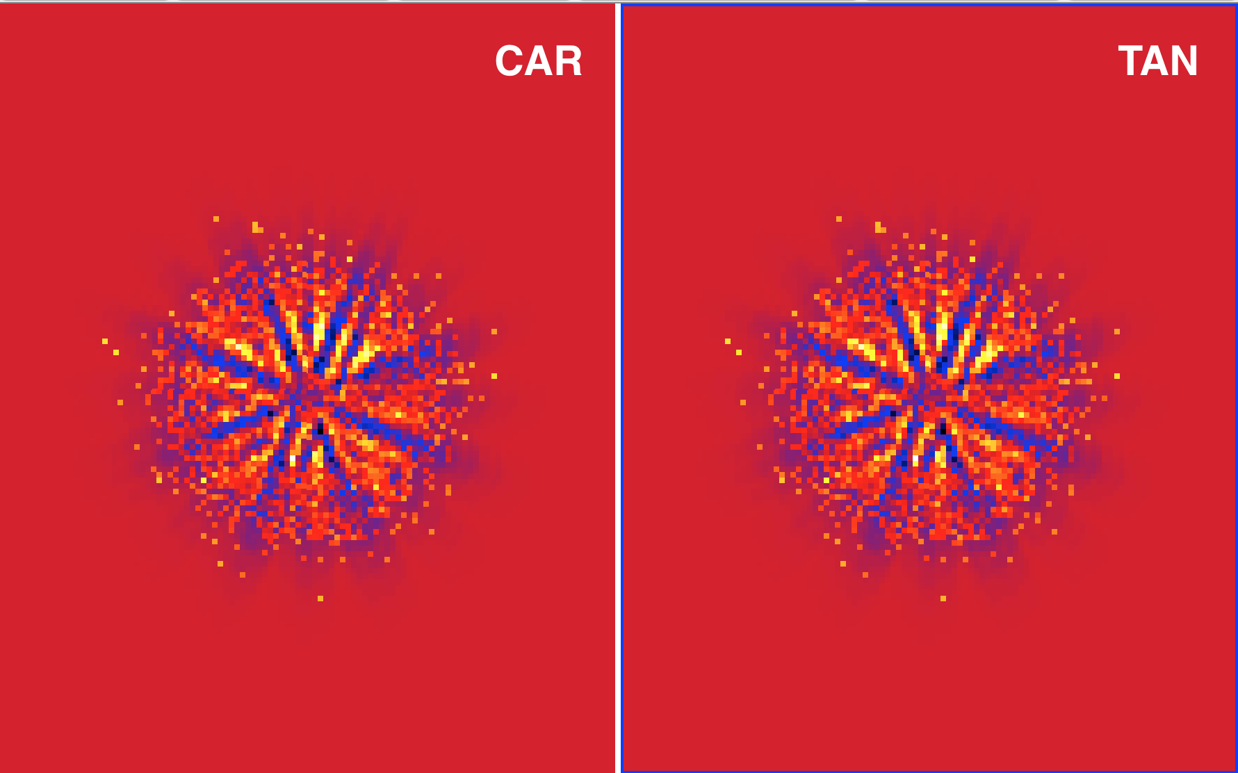
He sent a few residuals maps where some strange structures were present. I could reproduce the structures in the residual maps by simulating only source events (no background) for a simulation duration of 1 800 000 seconds. Below some residual maps for CAR and TAN projection with a spatial binning of 0.01 deg.

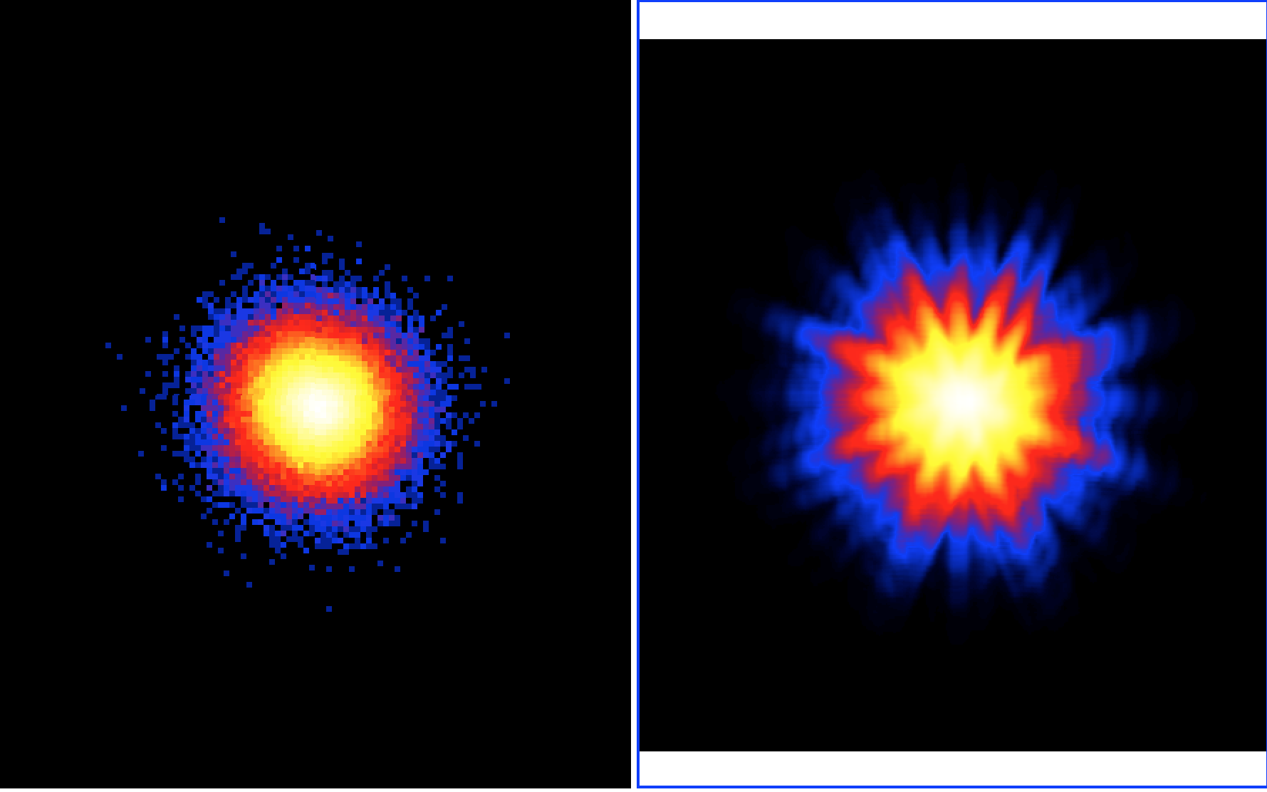
Below the corresponding counts map (left) and model map (right). The structure is only present in the model map while it is absent in the counts map. The problem seems to come from the modeling.
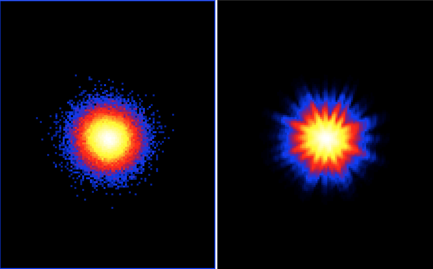
Note that the diffuse map has a very small spatial binning of 0.0035 deg, and since the spatial binning of the model map is only 0.01 deg maybe there is an issue with a too coarse binning (recall that the model is only sampled at the centre of the spatial bins).
Recurrence
No recurrence.
History
#1
 Updated by Knödlseder Jürgen almost 7 years ago
- File modmap_1800000_tan_0.001.png added
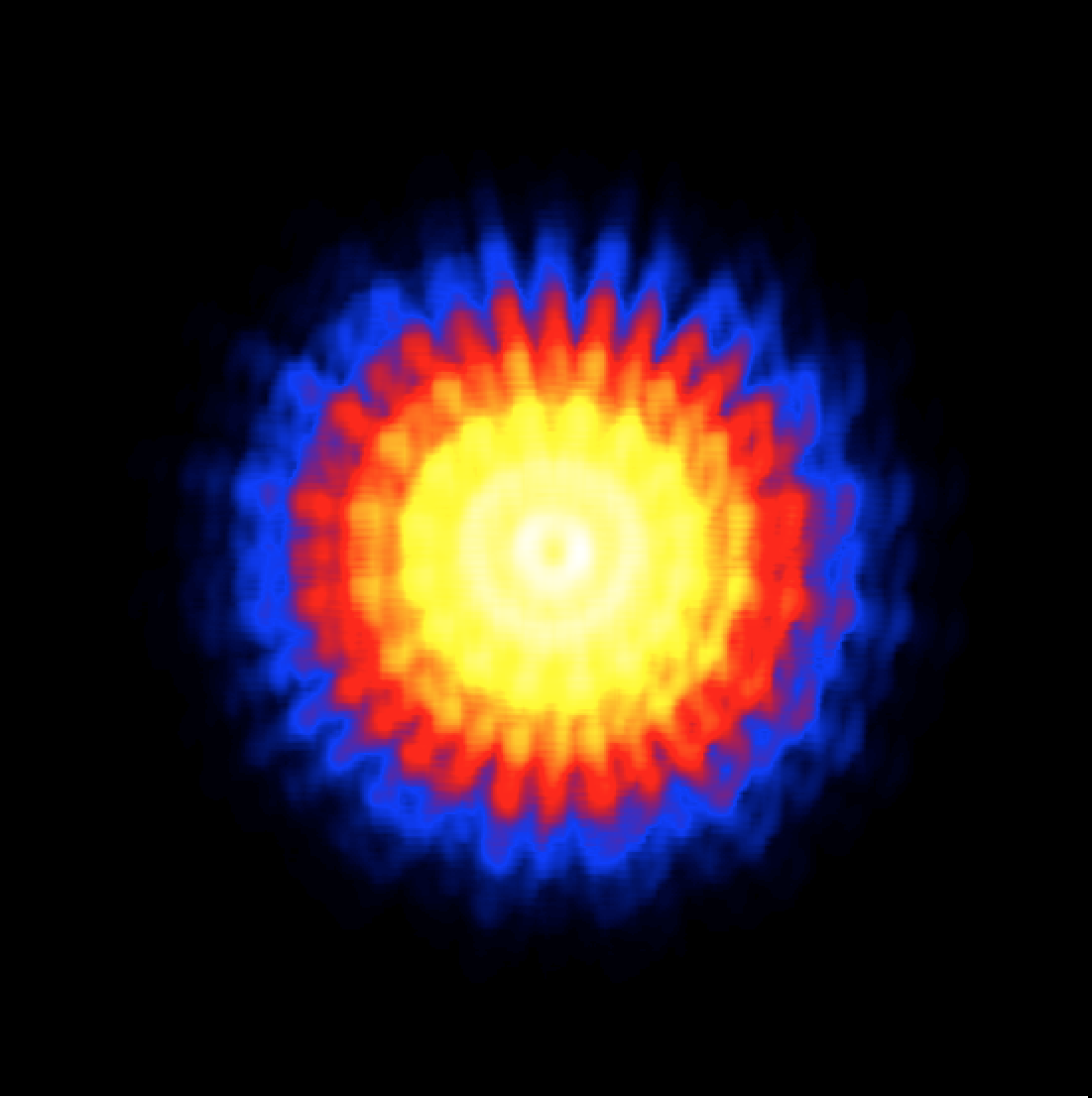
Computing the model cube with a sampling of 0.001 deg per pixel does not change the situation, hence it’s not a question of spatial sampling, as shown by the figure below.

#2
 Updated by Knödlseder Jürgen almost 7 years ago
- File modslice_1800000_tan_0.001_rho5_phi5.png added
- File modslice_1800000_tan_0.001_rho6_phi5.png added
- File modslice_1800000_tan_0.001_rho5_phi6.png added
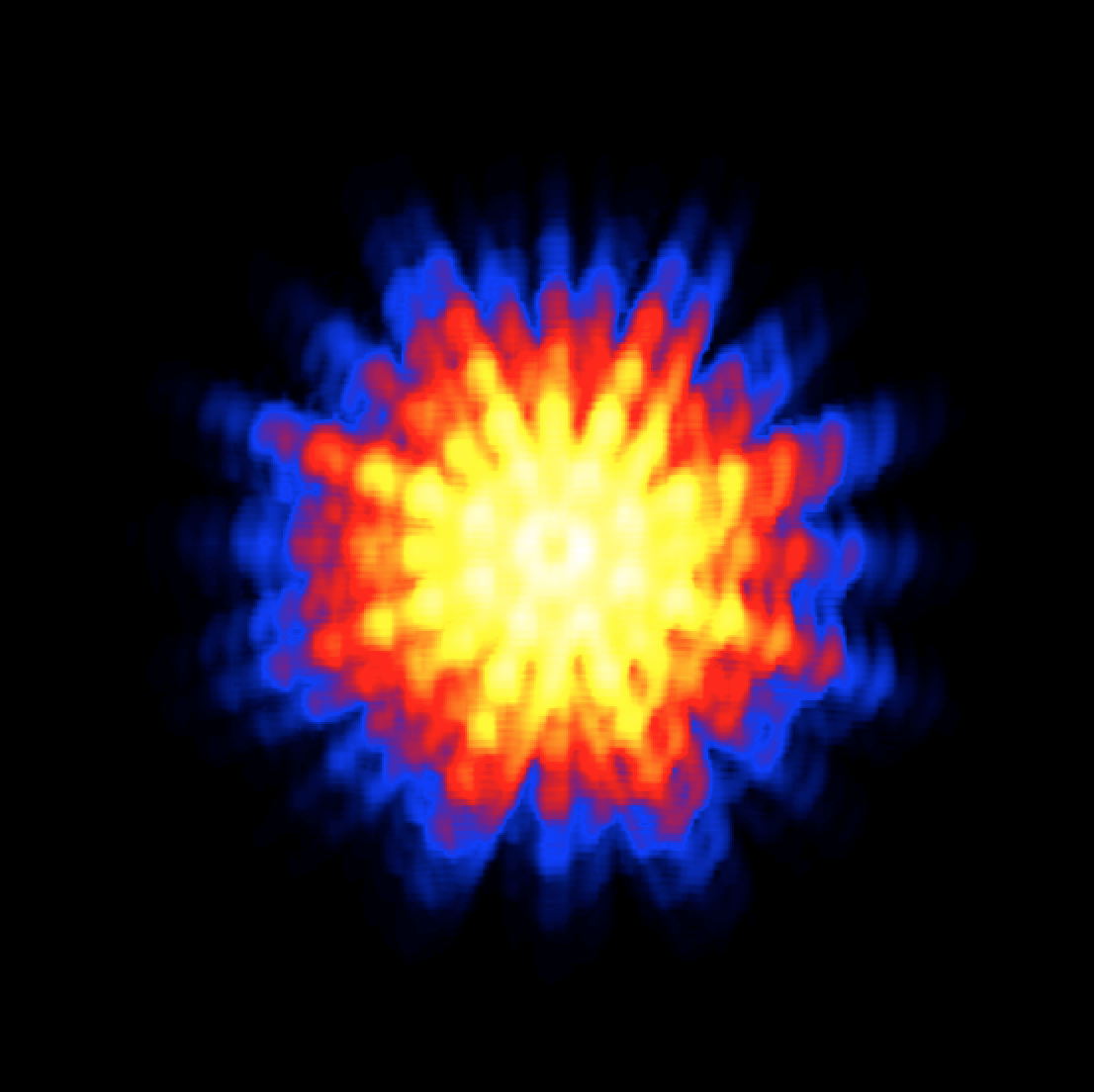
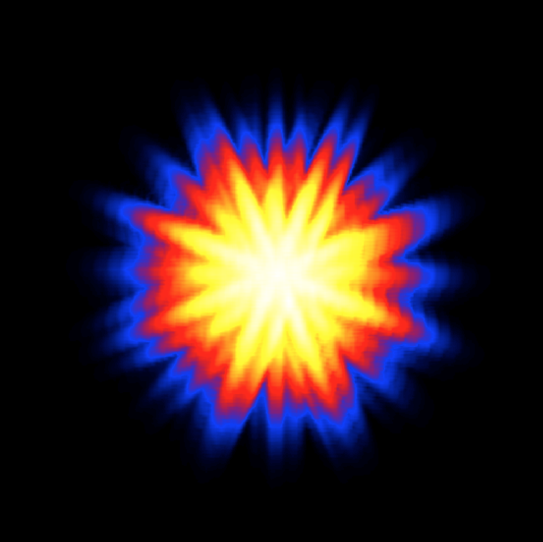
The problem comes from the discret integration steps in GCTAResponseIrf::irf_diffuse, with the number of Romberg iterations in rho and phi fixed to 5, which corresponds to 16 integration steps in radius and azimuth. Below the resulting model map in the 100-140 GeV bin for rho=phi=5 (left, default), rho=6, phi=5 (centre) and rho=5, phi=6. Increasing the number of steps in the radial direction smoothes the result radially, but still leads to a star-like structure. Increasing the number of steps in the azimuthal direction doubles the number of azimuthal steps and hence reduces the star-like appearance of the model.
 |
 |
 |
#3
 Updated by Knödlseder Jürgen almost 7 years ago
- File modelmap_20GeV_5x5_vs_8x8.png added
- Status changed from New to In Progress
- Assigned To set to Knödlseder Jürgen
- Target version set to 1.6.0
- % Done changed from 0 to 50
The problem arises in fact for sky maps that have a spatial resolution that is smaller than the CTA PSF. Due to the energy dependence this happens actually for many sky maps.
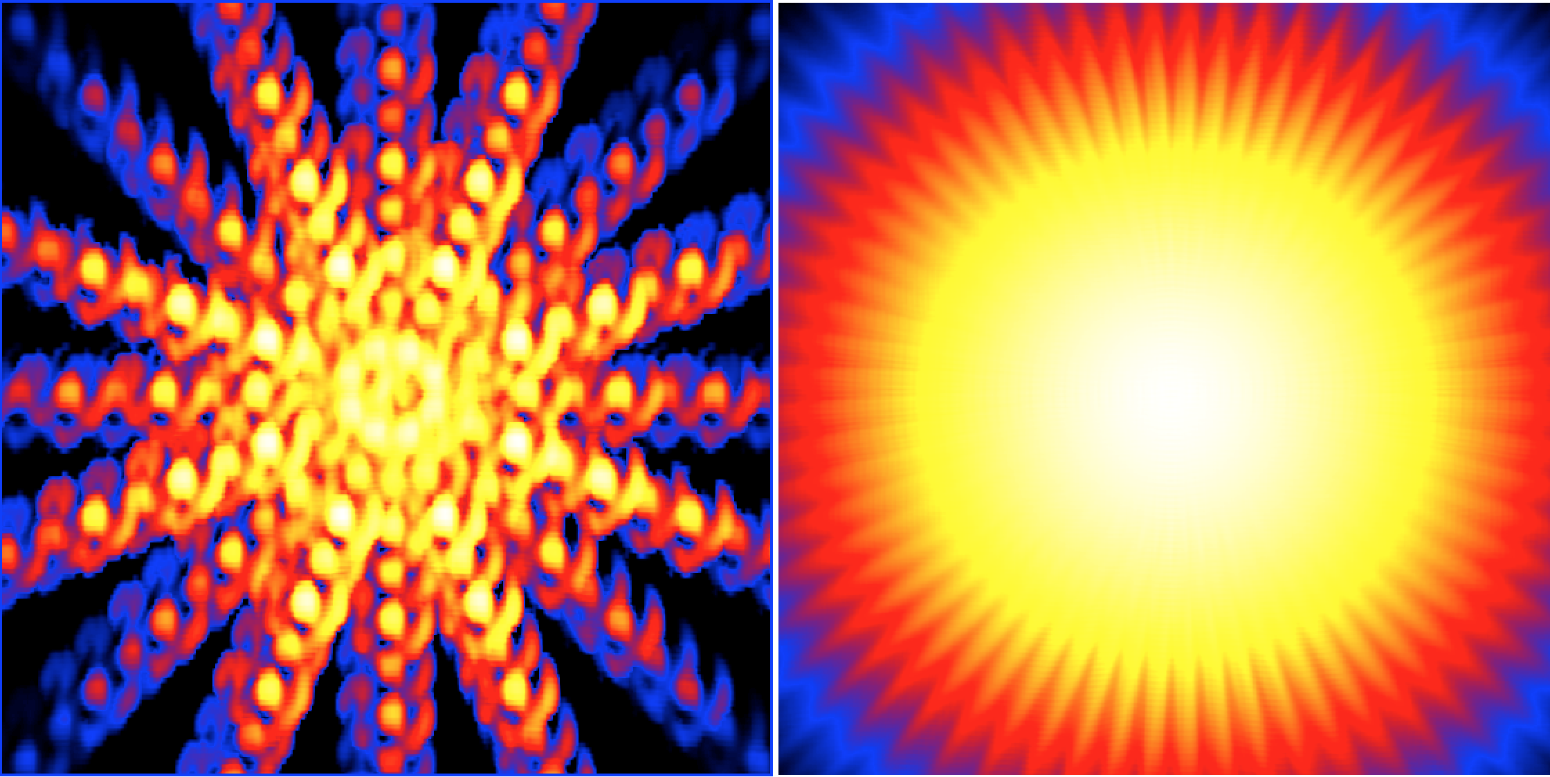
The left image below illustrated the problem. It shows a high-resolution model map for iter_rho=iter_phi=5 generate at 20 GeV, i.e. at an energy where the PSF is worst. At each point that was sampled, the image shows a little replica of the input sky map (a whirly structure around a spot). Increasing the number of iteration steps produces the image on the right. There is still some structure due to the discrete integration steps, but overall the model is now rather smooth.

To understand which integration precision is required, I did an event simulation and fitted the sky map using an unbinned analysis to the simulated events, varying the number of integration steps. An energy range of 20 GeV - 100 TeV was used. The results are summarized in the table below. For iter_rho=iter_phi=8 on the fit does no longer improve.
| iter_rho | iter_phi | TS | Prefactor | Index | CPU time |
| 5 | 5 | 4291.923 | 9.596e-18 +/- 3.612e-19 | 2.217 +/- 0.022 | 10.500 seconds |
| 6 | 6 | 4353.509 | 9.705e-18 +/- 3.645e-19 | 2.242 +/- 0.022 | 22.366 seconds |
| 7 | 7 | 4363.908 | 9.722e-18 +/- 3.649e-19 | 2.247 +/- 0.022 | 70.653 seconds |
| 8 | 8 | 4365.353 | 9.723e-18 +/- 3.650e-19 | 2.247 +/- 0.022 | 235.604 seconds |
| 9 | 9 | 4365.393 | 9.723e-18 +/- 3.650e-19 | 2.247 +/- 0.022 | 928.304 seconds |
I then implemented an algorithm where the actual integration precision depends on the spatial resolution of the map, computing iter_rho and iter_phi as follows:
iter_rho = log_2(rho_max/resolution) + 1
iter_phi = log_2(2*pi*rho/resolution) + 1
and constraining the number of iterations to the interval [5,8].
I then validated the algorithm using the simulation of Michele. The table below shows the results. For reference, the fit with the old scheme is shown in the first row. The next three rows show the results of the new scheme with a maximum number of iterations set to 7, 8 and 9, respectively. Also here, the TS value and fit parameters converge for a value of 8, hence we retain this value for the code. Note that with the new scheme, the TS value for the radio map are now larger than the values for the point source, radial disk and Gaussian disk models.
| Model | Scheme | TS | Prefactor | Index | Radius | CPU time |
| Radio map | 5x5 | 14100.852 | 8.138e-19 +/- 1.195e-20 | 2.277 +/- 0.011 | 7.291 s | |
| Radio map | max 7x7 | 14365.360 | 8.336e-19 +/- 1.212e-20 | 2.283 +/- 0.011 | 71.8693 s | |
| Radio map | max 8x8 | 14363.749 | 8.337e-19 +/- 1.212e-20 | 2.283 +/- 0.011 | 129.999 s | |
| Radio map | max 9x9 | 14363.853 | 8.337e-19 +/- 1.212e-20 | 2.283 +/- 0.011 | 158.459 s | |
| Point source | - | 13145.970 | 7.483e-19 +/- 1.150e-20 | 2.295 +/- 0.012 | 2.989 s | |
| Radial disk | - | 14307.270 | 8.272e-19 +/- 1.230e-20 | 2.285 +/- 0.011 | 0.047 +/- 0.001 | 32.247 s |
| Radial Gaussian | - | 14322.504 | 8.298e-19 +/- 1.241e-20 | 2.283 +/- 0.011 | 0.0243 +/- 0.0007 | 89.717 s |
#4
 Updated by Knödlseder Jürgen almost 7 years ago
- Status changed from In Progress to Feedback
- % Done changed from 50 to 100
Merged code into devel.
#5
 Updated by Knödlseder Jürgen almost 7 years ago
- Status changed from Feedback to Closed
