Action #2654

Correct handling of H.E.S.S. 3D energy dispersion IRFs
| Status: | Closed | Start date: | 07/31/2018 | |
|---|---|---|---|---|
| Priority: | Normal | Due date: | ||
| Assigned To: |  Knödlseder Jürgen Knödlseder Jürgen | % Done: | 100% | |
| Category: | - | |||
| Target version: | 1.6.0 | |||
| Duration: |
Description
Andreas Specovius reported some issues with the 3D IRF energy dispersion kludge when handling H.E.S.S. data. The smoothing-kludge does not work well for HESS data since the interpolation between optical phases leads to double peaks in the energy dispersion. There also seems to be an issue with the renormalization.

Recurrence
No recurrence.
History
#1
 Updated by Knödlseder Jürgen over 6 years ago
- File edisp_before.png added
- File edisp_after.png added
- % Done changed from 0 to 50
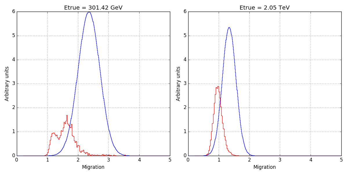
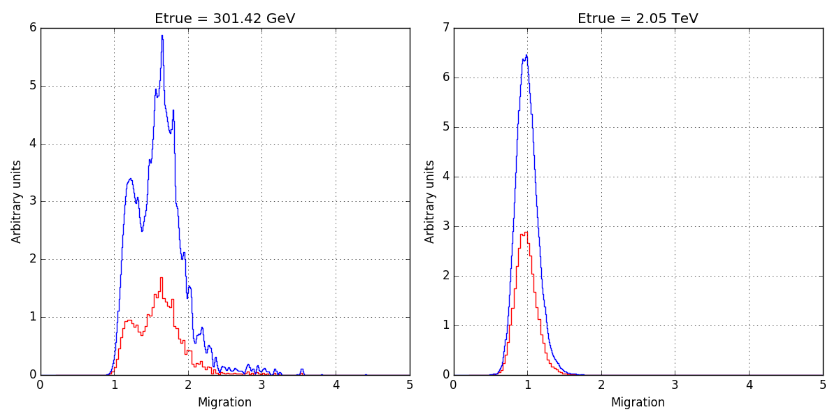
The energy dispersion kludge indeed distorts considerably the H.E.S.S. energy dispersion. The panels below show the energy dispersion as provided in the FITS file hess_edisp_2d_047802.fits as red histograms and the energy dispersion as returned by GCTAEdisp2D as blue histograms. Left panel is with the energy dispersion kludge, right panel is without the energy dispersion kludge.
 |
 |
Note that the internal GCTAEdisp2D normalization still leads to a different magnitude of the energy dispersion, but that internal normalization is needed since the integral of the GCTAEdisp2D operator over log(E_obs) should be unity. To check this I computed the integrals using a simple Python code
logEsrc = math.log10(etrues[ietrue])
migs    = [0.01*i+0.01 for i in range(500)]
sum     = 0.0
for mig in migs:
    logEobs     = math.log10(mig) + logEsrc
    logEobs_max = math.log10(mig+0.005)
    logEobs_min = math.log10(mig-0.005)
    dlogEobs    = logEobs_max-logEobs_min
    value       = edisp2D(logEobs, logEsrc, 0.0)
    sum        += value * dlogEobs
print('Sum of edisp2D %f' % sum)
The results for both histograms are
Sum of edisp2D 1.000108
Sum of edisp2D 0.999869
while without the internal normalisation they are
Sum of edisp2D 0.281121
Sum of edisp2D 0.445356
I guess that HAP fills the histograms so that the integral over the migration is unity, but the normalisation needed is that the integral over the log10 of reconstructed energy is unity.
So my conclusion is that the normalization is done correctly, and you should keep it to get the correct fit results.
#2
Updated by Knödlseder Jürgen over 6 years ago
- Status changed from New to Feedback
- % Done changed from 50 to 100
I added some more Doxygen documentation to the GCTAEdisp2D class (and also the other energy dispersion classes) to clarify the mathematics. From my side this issue is done (well, code still needs to be merged in). I put the status to Feedback.
#3
 Updated by Specovius Andreas over 6 years ago
Knödlseder Jürgen wrote:
Note that the internal
GCTAEdisp2Dnormalization still leads to a different magnitude of the energy dispersion, but that internal normalization is needed since the integral of theGCTAEdisp2Doperator over log(E_obs) should be unity.
I guess that HAP fills the histograms so that the integral over the migration is unity, but the normalisation needed is that the integral over the log10 of reconstructed energy is unity.So my conclusion is that the normalization is done correctly, and you should keep it to get the correct fit results.
Indeed the H.E.S.S. energy dispersion is normalized so that the integral over the migration axis is unity.
As you described, the internal ctools normalization may hence make sense!
The only point I am still a bit worried about is whether the integral algorithm works correctly concerning the double peak structure observed in the H.E.S.S. edisp and also concerning isolated nonzero bins.
Do you have experience about that or has this been tested yet?
#4
Updated by Knödlseder Jürgen over 6 years ago
- File integration-issues.png added
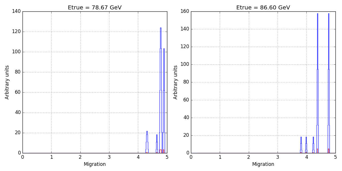
I made a quick check of the file you sent me using the simple algorithm from above. Below the list where the differences from 1 are larger than 1%:
0.0 deg   0.07 TeV sum: 0.025961
0.0 deg   0.08 TeV sum: 1.197912
0.0 deg   0.09 TeV sum: 1.295726
0.0 deg   0.10 TeV sum: 1.068557
0.0 deg   0.13 TeV sum: 1.020230
0.0 deg  95.32 TeV sum: 1.012170
0.5 deg   0.07 TeV sum: 0.025961
0.5 deg   0.08 TeV sum: 1.197912
0.5 deg   0.09 TeV sum: 1.295726
0.5 deg   0.10 TeV sum: 1.068557
0.5 deg   0.13 TeV sum: 1.020230
0.5 deg  95.32 TeV sum: 1.012170
1.0 deg   0.07 TeV sum: 0.025961
1.0 deg   0.08 TeV sum: 1.197912
1.0 deg   0.09 TeV sum: 1.295726
1.0 deg   0.10 TeV sum: 1.068557
1.0 deg   0.13 TeV sum: 1.020230
1.0 deg  95.32 TeV sum: 1.012170
1.5 deg   0.07 TeV sum: 0.025961
1.5 deg   0.08 TeV sum: 1.197912
1.5 deg   0.09 TeV sum: 1.295726
1.5 deg   0.10 TeV sum: 1.068557
1.5 deg   0.13 TeV sum: 1.020230
1.5 deg  95.32 TeV sum: 1.012170
2.0 deg   0.07 TeV sum: 0.025961
2.0 deg   0.08 TeV sum: 1.197912
2.0 deg   0.09 TeV sum: 1.295726
2.0 deg   0.10 TeV sum: 1.068557
2.0 deg   0.13 TeV sum: 1.020230
2.0 deg  95.32 TeV sum: 1.012170
2.5 deg   0.07 TeV sum: 0.025961
2.5 deg   0.08 TeV sum: 1.197912
2.5 deg   0.09 TeV sum: 1.295726
2.5 deg   0.10 TeV sum: 1.068557
2.5 deg   0.13 TeV sum: 1.020230
2.5 deg  95.32 TeV sum: 1.012170
So there are differences up to almost 30%, but they occur at very low energy. The plot below shows that those arise when only a few bins are set in the histogram.
#5
Updated by Knödlseder Jürgen about 6 years ago
- Status changed from Feedback to Closed