Support #3160

Residual cosmic-ray background flux with ctmodel and ctexpcube
| Status: | In Progress | Start date: | 02/19/2020 | ||
|---|---|---|---|---|---|
| Priority: | Normal | Due date: | |||
| Assigned To: | - | % Done: | 50% | ||
| Category: | - | ||||
| Target version: | - | ||||
| Duration: |
Description
I would like to address a result which I have obtained with ctools 1.5.2 and prod3b-v1 IRFs (South_z20_average_50h):
I intend to derive the expected residual cosmic-ray background flux in the context of CTA’s Galactic centre survey. I attach the necessary observation definition file. To save computation time, I want to use ctmodel (model file: 'cr.xml’) for an energy range from 30 GeV to 100 TeV and 100 logarithmically-spaced spectral bins. The output cosmic-ray counts cube should then be divided by the exposure per spectral and spatial bin. Such an exposure map may be derived with ctexpcube and the same observation and binned cube file.
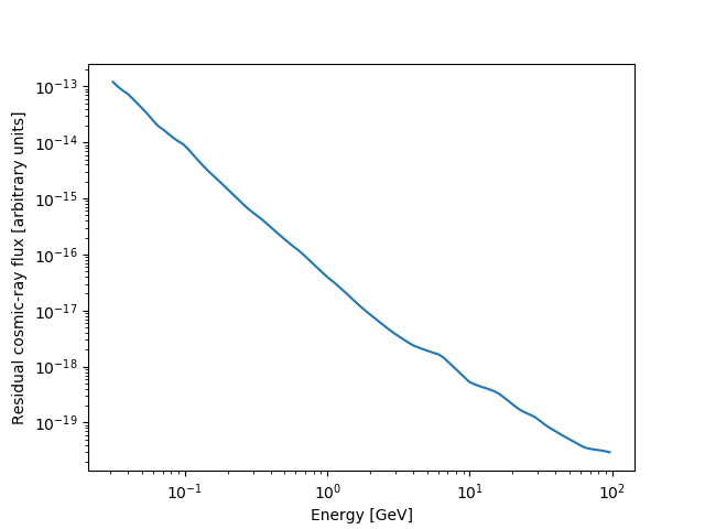
According to my understanding, the exposure map contains the exposure in units of [m^-2 s^-1] (correct?) at all energy bin edges (in total 101). Hence, I define an interpolation function to obtain the exposure at any energy within the predefined range. If I remember correctly, ctmodel uses the central energy of the respective energy bin to calculate the model counts. With that information in mind, I divide counts by exposure (ensuring that a division by zero is impossible) and plot the resulting flux per energy bin as shown in the figure (x-axis: energy in GeV, y-axis: residual cosmic-ray background flux in arbitrary units).
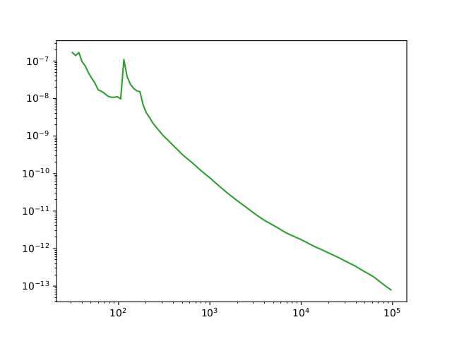
I do not understand the very strange behaviour around a few hundred GeV which clearly seems to indicate that something went wrong. I attach a python script which performs the ctools commands and the calculation of the final flux figure. Do you have a feeling what might be the issue here?
cr_flux_from_exposure.py  - minimal python script to generate count cubes and further calculations
(2.12 KB)
- minimal python script to generate count cubes and further calculations
(2.12 KB)
bin_generic_GC_survey_ROI_12x12deg_100EBINS_0p01deg.fits.gz - binned counts cube to extract general cube definition (11.5 MB)
obs_CTA_GC_survey_ROI_5deg.xml
- observation file (CTA Galactic centre survey)
(5.48 KB)
cr.xml
- model file for cosmic-ray background
(534 Bytes)
cosmic_ray_flux_using_ctmodel_and_ctexpcube.png (19.6 KB)
my_interp.png (26.1 KB)
bin_200.png (25.8 KB)
bin_600.png (26.2 KB)
no_0exp.png (25.9 KB)
cr_flux_from_exposure.py
(4.11 KB)


Recurrence
No recurrence.
History
#1
 Updated by Tibaldo Luigi almost 5 years ago
- File my_interp.png added
- File bin_200.png added
- File bin_600.png added
- File no_0exp.png added
- File cr_flux_from_exposure.py added
- Status changed from New to In Progress
- % Done changed from 0 to 50
Warning! Sorry, I realized when posting the figures that I had made a mistake, the units in the x-axis label should be TeV, not GeV
Hi Christopher,
sorry for taking so long, I needed to play around for a little to understand what was going on.
I think your results are essentially correct, and the discontinuities you see are the result of the fact that you study a large region of the sky, in which, for the observation strategy implemented, the instrumental energy threshold varies quite a lot as a function of the direction in the sky (the instrument threshold is at the lower-energy end considered in the analysis, 30 GeV, about a couple of degrees around the center of the region, and it increases up to a hundred GeV closer to the borders).
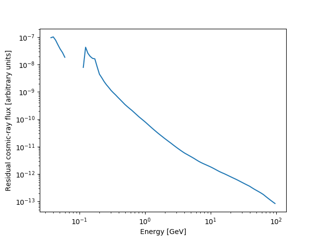
In the process to understand the problem I implemented my own version of the exposure interpolation (main difference: power-law piece-wise interpolation rather than linear piece-wise interpolation as you were doing). The resulting spectrum still has the same features.

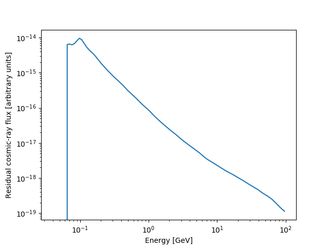
I checked a few individual bins. You can see very well that in each spatial bin the CR spectrum is reasonably smooth, but that the threshold varies significantly

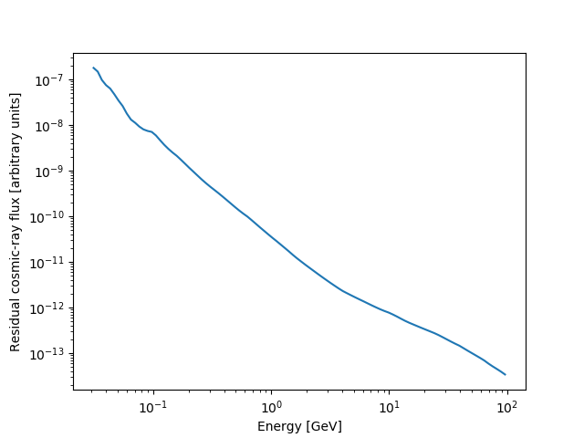
Below you can see an integrated spectrum over the region where the instrument threshold coincides with the analysis threshold of 30 GeV, which, again, is rather smooth.

Thus, as anticipated at the beginning, I think that the energies at which you see discontinuities in your spectrum are due to some parts of the region reaching the instrument threshold, or, in practice, to a bunch of new pixels being included in the total flux.
In summary, nothing wrong, what you obtained is indeed the total CR flux over the region you chose for the pointing strategy considered. You should not be surprised by the comparison with the background rate in the CTA performance page, because that shows the spectrum over a small 0.2 deg region close to the pointing direction.
The script with my mods/additions is also attached.
If you explain a bit more what you aims are I may help you to figure out how to proceed.
Cheers, Luigi
#2
 Updated by Eckner Christopher almost 5 years ago
Hi Luigi,
Thanks for having a look into this matter. To me, your explanation makes sense, and I have already had a suspicion in that direction.
As concerns the aim of this exercise, I am not sure how to proceed. Intentionally, such a flux plot should appear in the 'Dark Matter in the Galactic Centre’ CTA Consortium paper. Of course, not just the residual cosmic-ray background but also the remaining astrophysical and dark matter components. The plot we are showing right now is referring to model predictions. We thought that it would be nicer to show the eventually expected flux levels after the convolution with CTA’s IRFs for the full ROI of 12°x12°. This way, theorists could digitise the numbers and make rough estimates if needed.
We could, of course, only for this plot shrink the reference ROI to generate a plot without these spikes (analogous to your last plot). On the other hand, showing the fluxes with spikes would hardly get the blessings from the CTA Consortium, right? Hence, we now display counts per energy bin for each component. One can still grasp the relative strength of each component, but we might disappoint some theorists.
Do you have a better idea?
Best,
Christopher