Feature #4209

Study implementation of an alternative BGDLIX algorithm for COMPTEL
| Status: | In Progress | Start date: | 02/10/2023 | ||
|---|---|---|---|---|---|
| Priority: | Normal | Due date: | |||
| Assigned To: |  Knödlseder Jürgen Knödlseder Jürgen | % Done: | 70% | ||
| Category: | - | ||||
| Target version: | 2.1.0 | ||||
| Duration: |
Description
The BGDLIX algorithm takes advantage of the fact that the event distribution in the DRE follows to first order the shape of the DRG. This however only holds for a constant event rates. As CGRO orbits the Earth the radiation environment changes continuously, leading to an ever changing event rate (see Weidenspointner’s PhD thesis). In addition there are long-term variations that related to orbital altitude. Plausibly, the event rate variations are energy dependent, e.g. through the build-up of long-lived isotopes (e.g. Fig. 4.47 in Weidenspointner’s PhD thesis).
At the same time, the DRG shape changes due to the Earth horizon cut, which presents a second time dependence. This may lead to significant differences between the DRE and DRG, which may explain why residuals of the BGDLIX method tend to be stronger when the Earth is in the field of view.
An alternative BGDLIX algorithm could make use of a special energy dependent DRW dataset that is the DRG which includes the time and energy dependent event rate, for example on a superpacket basis, or a longer time interval if there are not enough events within a superpacket to derive a meaningful event rate.
The DRW should finally be normalised per Phibar layer to the DRE, so that DRW can be added up in the comobsadd step.
In the alternative BGDLIX algorithm, the DRW would be used instead of the DRG.
event-rate-zoom.png (149 KB)
event-rate.png (177 KB)
event-rate-zoom-5min-10bins-norm.png (305 KB)
event-rate-zoom-5min-10bins.png (255 KB)
event-rate-zoom-2min-3bins-norm.png (169 KB)
event-rate-zoom-2min-3bins.png (147 KB)
event-rate-vp001.0-3h-3bins.png (219 KB)
event-rate-vp201.0-3h-3bins.png (198 KB)
event-rate-vp301.0-3h-3bins.png (176 KB)
event-rate-vp401.0-3h-3bins.png (212 KB)
event-rate-vp501.0-3h-3bins.png (208 KB)
event-rate-vp601.1-3h-3bins.png (230 KB)
event-rate-vp625.0-3h-3bins.png (263 KB)
event-rate-vp625.0-6h-10bins.png (432 KB)
event-rate-vp631.1-3h-3bins.png (201 KB)
event-rate-vp631.1-6h-10bins.png (356 KB)
event-rate-vp001.0-5m-three.png (206 KB)
event-rate-vp201.0-5m-three-zoom.png (243 KB)
event-rate-vp201.0-5m-three.png (319 KB)
event-rate-vp301.0-5m-three-zoom.png (224 KB)
event-rate-vp301.0-5m-three.png (319 KB)
event-rate-vp401.0-5m-three-zoom.png (235 KB)
event-rate-vp401.0-5m-three.png (236 KB)
event-rate-vp501.0-5m-three.png (240 KB)
event-rate-vp501.0-5m-three-zoom.png (238 KB)
event-rate-vp001.0-5m-three-zoom.png (190 KB)
event-rate-vp625.0-5m-three.png (251 KB)
event-rate-vp625.0-5m-three-zoom.png (237 KB)
phibar-impact.png (298 KB)
phibar-impact-eha.png (327 KB)
phibar-impact-eha-1min.png (263 KB)
phibar-impact-eha-2min.png (255 KB)
phibar-impact-eha-3min.png (228 KB)
phibar-impact-high-5min.png (182 KB)
phibar-impact-mid-5min.png (230 KB)
phibar-impact-low-5min.png (197 KB)
res_ehacorr_max10.png (506 KB)
res_noehacorr.png (499 KB)
res_ehacorr_max100.png (506 KB)
res_ehacorr_max1000.png (506 KB)
res_ehacorr_max10_150sec.png (506 KB)
res_ehacorr_max10_75sec.png (506 KB)
logl-profiles-vp0518.5.png (93.1 KB)
fit_eventrates.py  (14.4 KB)
res_binned_vp0518.5_bgdlixf-vetorate.png (506 KB)
residuals0.png (216 KB)
residuals1.png (182 KB)
residuals2.png (209 KB)
residuals3.png (218 KB)
residuals0-gauss1h.png (205 KB)
residuals1-gauss1h.png (172 KB)
residuals2-gauss1h.png (209 KB)
residuals3-gauss1h.png (217 KB)
corrected1-fc1-gauss1h-1st.png (166 KB)
corrected1-fc1-gauss1h-2nd.png (191 KB)
corrected1-fc1-gauss1h-3rd.png (184 KB)
corrected1-fc1-gauss1h-4th.png (184 KB)
corrected2-fc1-gauss1h-1st.png (179 KB)
corrected2-fc1-gauss1h-2nd.png (221 KB)
corrected2-fc1-gauss1h-3rd.png (244 KB)
corrected1-fc1-gauss1h-5th.png (188 KB)
corrected0-fc1-gauss1h-1st.png (217 KB)
corrected0-fc1-gauss1h-2nd.png (254 KB)
corrected3-fc1-gauss1h-1st.png (204 KB)
corrected3-fc1-gauss1h-2nd.png (265 KB)
corrected3-fc1-gauss1h-3rd.png (281 KB)
corrected3-fc1-gauss1h-4th.png (296 KB)
corrected3-fc1-gauss1h-5th.png (306 KB)
corrected2-fc1-gauss1h-4th.png (249 KB)
corrected2-fc1-gauss1h-5th.png (257 KB)
corrected0-fc1-gauss1h-4th.png (259 KB)
corrected0-fc1-gauss1h-3rd.png (259 KB)
corrected0-fc1-gauss1h-5th.png (259 KB)
res_binned_vp0518.5_bgdlixf-vetorate-activ5-1h.png (506 KB)
drw-rates.png (986 KB)


Recurrence
No recurrence.
History
#1
 Updated by Knödlseder Jürgen about 2 years ago
- File event-rate-zoom.png added
- File event-rate.png added
- Status changed from New to In Progress
- % Done changed from 0 to 10
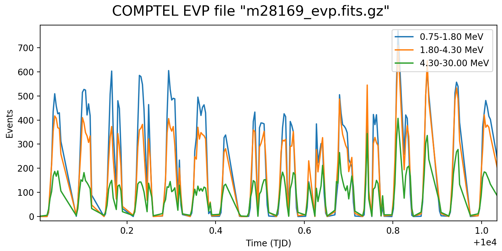
The plots below show the event rate variations as function of energy for VP0001. The rates were determined by accumulating the number of events in 2 minutes time windows. Obviously, the event rate changes depend strongly on energy, as shown in the right-hand panel which is a zoom into three orbits.
 |
 |
It is obvious that the energy-dependent event rate cannot be determined on the level of a superpacket, at least a few minutes are needed. Since the CGRO orbit is about 90 min, the accumulation time cannot be too long as otherwise the event rate variations get smeared out. Maybe 5 min would be a more reasonable time scale, yet the noise in the event rate depends of course also on the energy binning. Eventually, the noise is maybe not really an issue, since the DRG will not change a lot on minute times scales. Maybe I should try for the finest energy binning possible (e.g. the 30 bins used for the Crab analysis) and see at what time scale at least 5-10 events are in each energy bin. Alternatively, broader energy bins could be used for the event rate determination, and eventually a 2D bilinear interpolation could be used to assess the DRG weighting for a given superpacket time.
#2
Updated by Knödlseder Jürgen about 2 years ago
- File event-rate-zoom-5min-10bins-norm.png added
- File event-rate-zoom-5min-10bins.png added
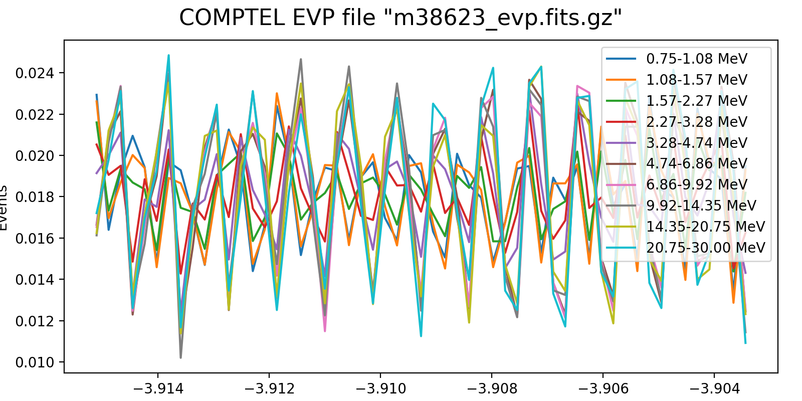
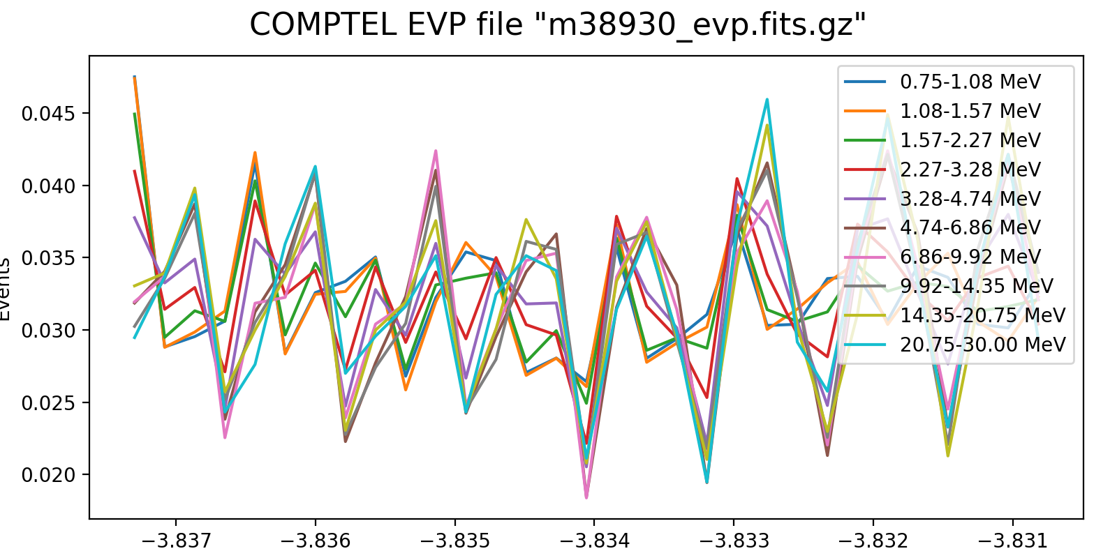
To better understand the strategy I redid the rate plotting for 10 logarithmically spaced energy bins and zoomed on the same zone as before. Below the result, with on the left the 5-min event rate and the right the event-rate normalised to the same number of total events. It’s not very clear whether actually an important energy dependency exists (at least on the short term).
 |
 |
#3
Updated by Knödlseder Jürgen about 2 years ago
- File event-rate-zoom-2min-3bins-norm.png added
- File event-rate-zoom-2min-3bins.png added
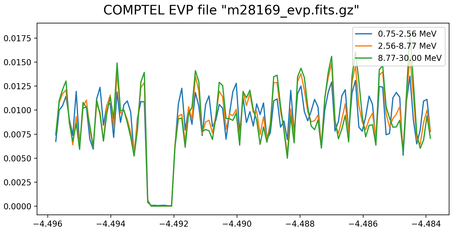
Maybe the energy dependent variability may come in on longer time scales, at short times there are probably not enough events to make this visible. Hence the strategy could be to use the full energy range for the short term variability and to merge it with an energy-dependent long-term trend. Below the results for 2-min rates for three energy intervals. Some energy-dependent trends may be visible, in particular in the last orbit shown.
 |
 |
#4
Updated by Knödlseder Jürgen about 2 years ago
- File event-rate-vp001.0-3h-3bins.png added
- File event-rate-vp201.0-3h-3bins.png added
- File event-rate-vp301.0-3h-3bins.png added
- File event-rate-vp401.0-3h-3bins.png added
- File event-rate-vp501.0-3h-3bins.png added
- File event-rate-vp601.1-3h-3bins.png added
- File event-rate-vp625.0-3h-3bins.png added
- File event-rate-vp625.0-6h-10bins.png added
- File event-rate-vp631.1-3h-3bins.png added
- File event-rate-vp631.1-6h-10bins.png added
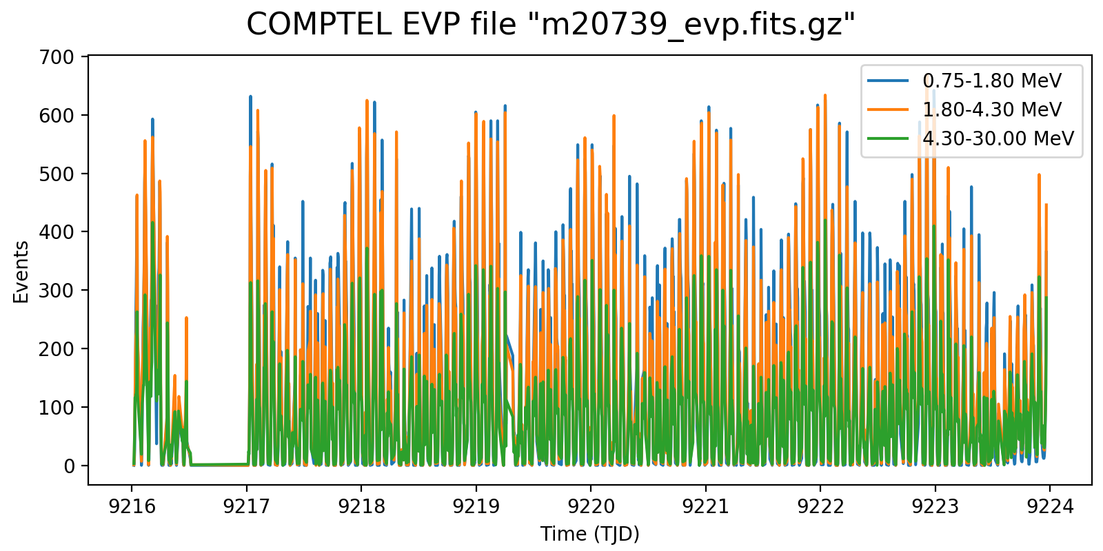
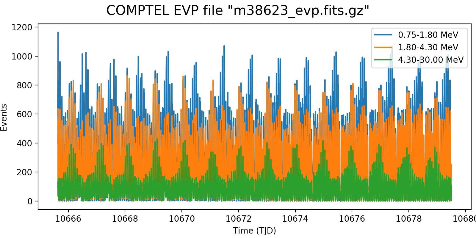
Event rate variation on a 3h timescale for one VP in each mission phase and two VP after the second reboost. While at the beginning the variation in all energy bins are synchronised, they diverge for later phases, and particularly after the second reboost. This is in line with the observation (cf. Weidenspointner PhD thesis) of gradual build-up of long-lived radioisotopes, in particular 22Na (his figure 4.47). Note also that Weidenspointner mentions that the activity during long-lived radio isotopes was at a minimum during phase 2, which may explain why there is very little energy dependence for VP 201 and 301.
1.0  |
201.0  |
301.0 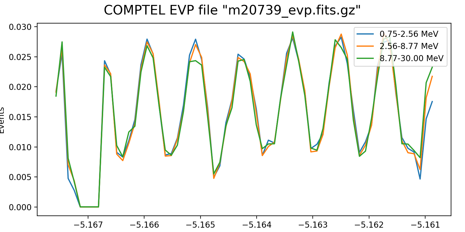 |
401.0  |
501.0  |
601.1 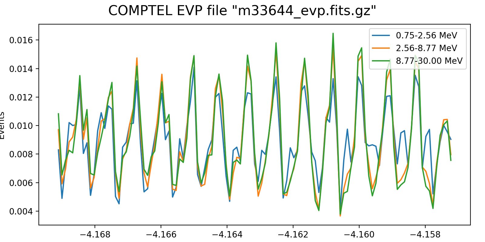 |
625.0  |
631.1  |
Below I investigated the behaviour after the second reboost using 10 energy bins and a longer time scale of 6 hours. There is a clear change in behaviour for <4.7 MeV, as recognised also by Weidenspointner (he states a change at 4.3 MeV). This could point towards a model where the background rate is composed of a prompt and a delayed component, where the prompt component is traced by the high-energy event rate (e.g. above 4.3 MeV; see below), while the delayed component is traced by the residual low-energy rate.
625.0  |
631.1  |
#5
Updated by Knödlseder Jürgen about 2 years ago
- CGRO telemetry limits number of events transmitted to 48 events per 2.048 sec long packet
- The background is characterised by three distinct energy ranges: 0.8-4.3 MeV (nuclear line emission), 4.3-9 MeV (nuclear continuum emission), 9-30 MeV
- A large fraction of the instrumental background is due to prompt processes
- Below 4.3 MeV (and particularly below 1.8 MeV) the background is strongly influenced by long-lived components
- Above 4.3 MeV no signifiant long-lived background components are present
- Long-lived isotopes are activated during SAA passages
- CGRO orbit is such that it passes through SAA in 7 consecutive orbits and then avoids SAA in next 7 orbits. 24Na activity is building up during SAA passages, and decaying when SAA is avoided.
#6
Updated by Knödlseder Jürgen about 2 years ago
- File event-rate-vp001.0-5m-three.png added
- File event-rate-vp201.0-5m-three-zoom.png added
- File event-rate-vp201.0-5m-three.png added
- File event-rate-vp301.0-5m-three-zoom.png added
- File event-rate-vp301.0-5m-three.png added
- File event-rate-vp401.0-5m-three-zoom.png added
- File event-rate-vp401.0-5m-three.png added
- File event-rate-vp501.0-5m-three-zoom.png added
- File event-rate-vp501.0-5m-three.png added
- File event-rate-vp001.0-5m-three-zoom.png added
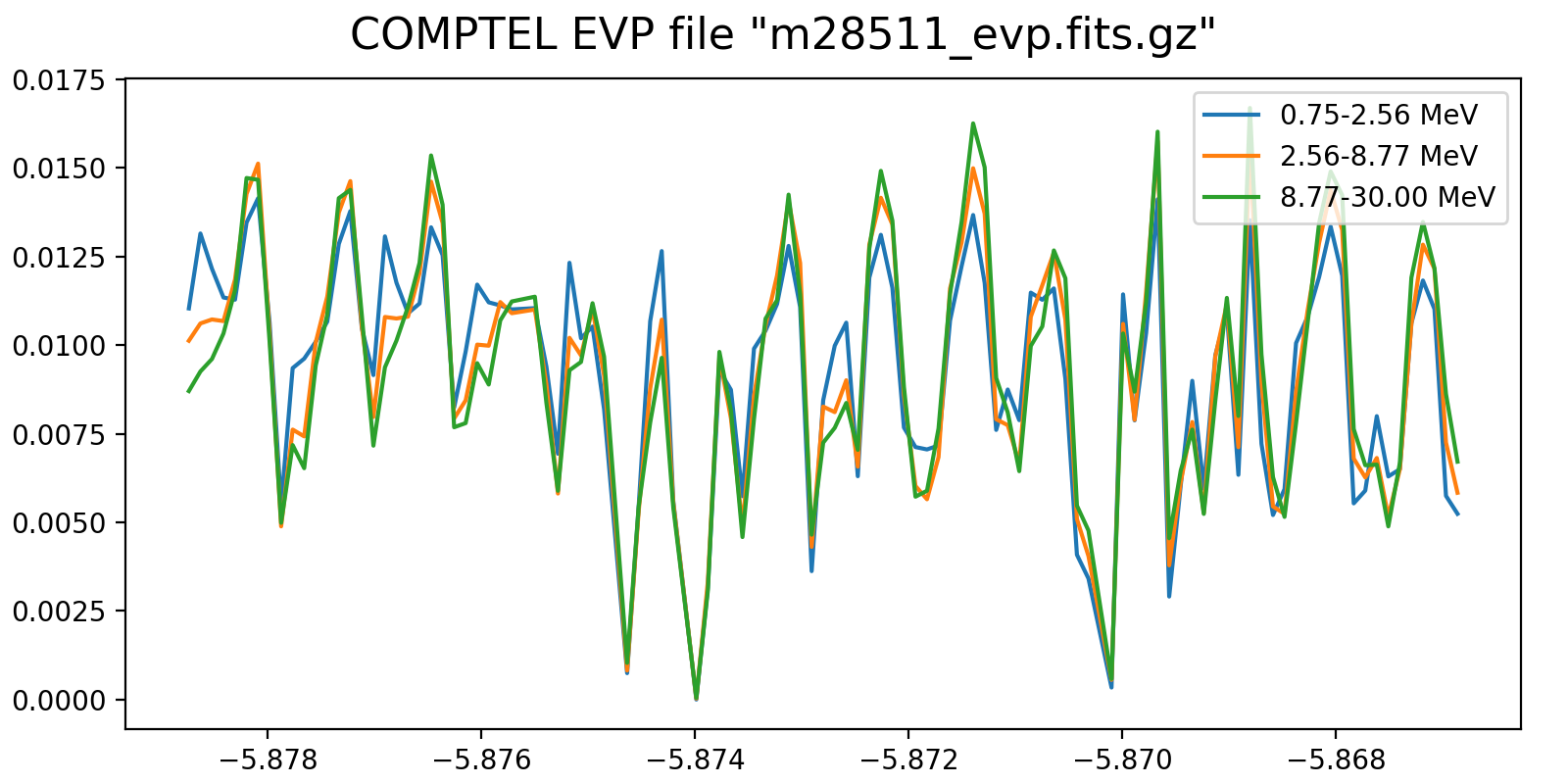
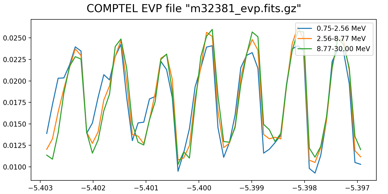
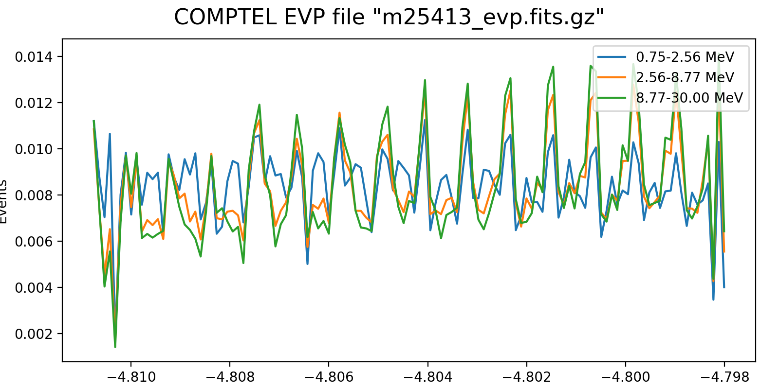
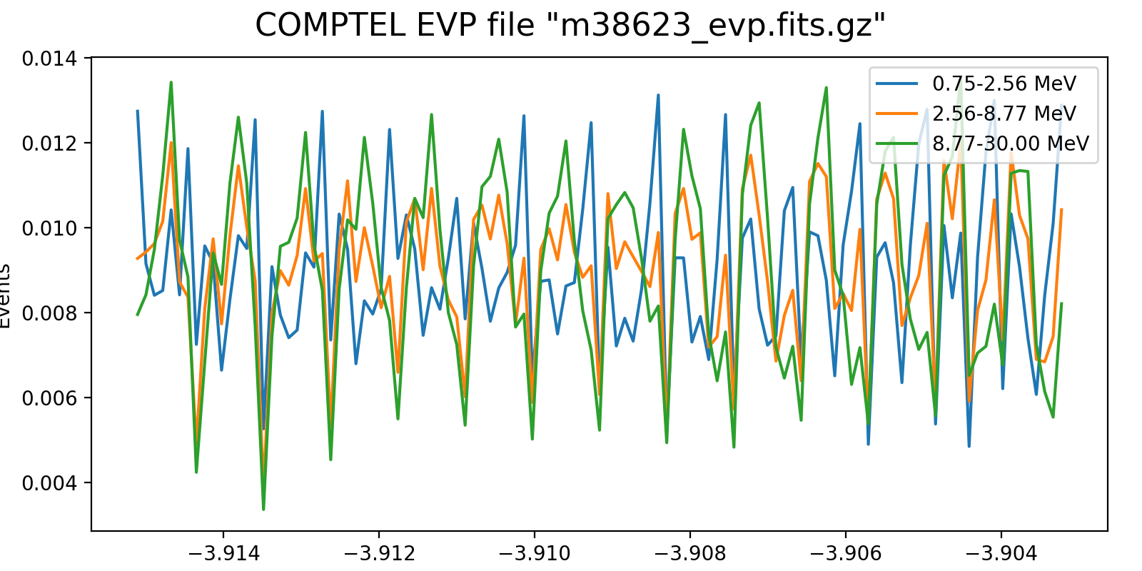
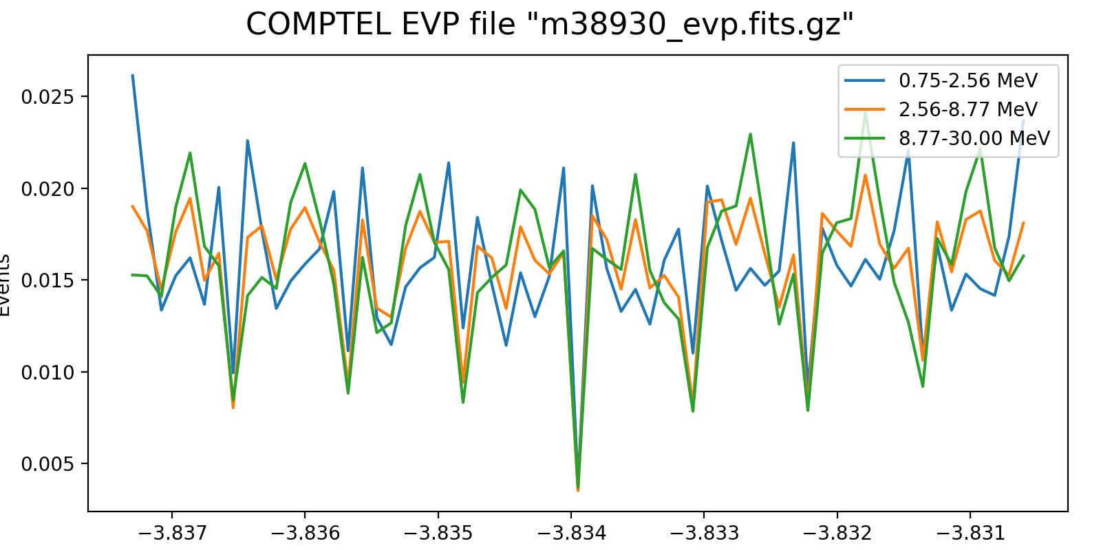
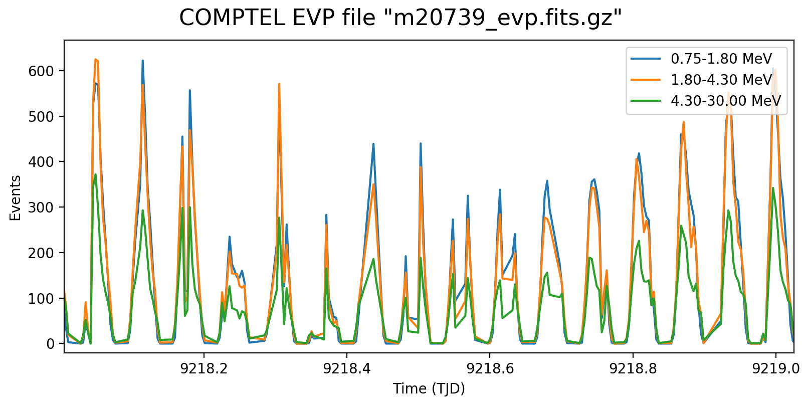
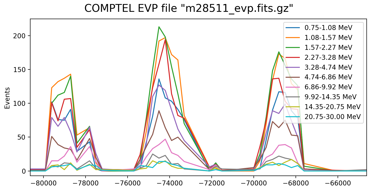
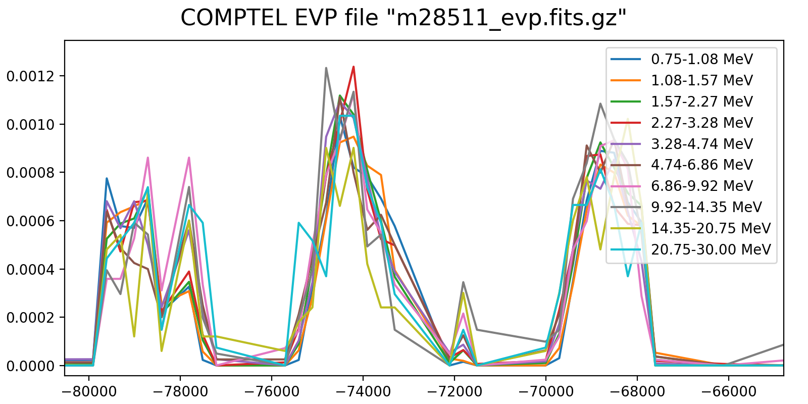
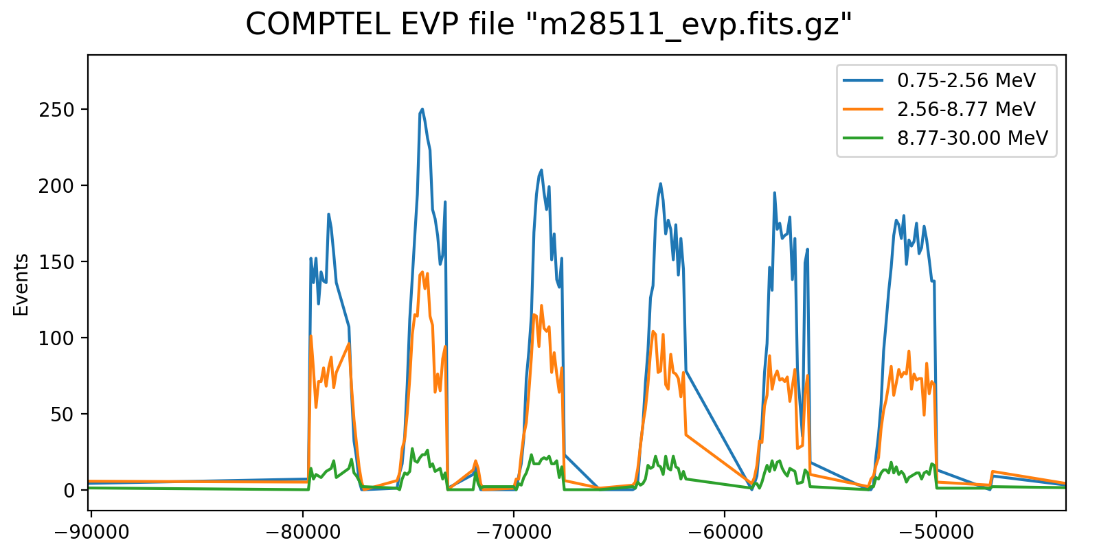
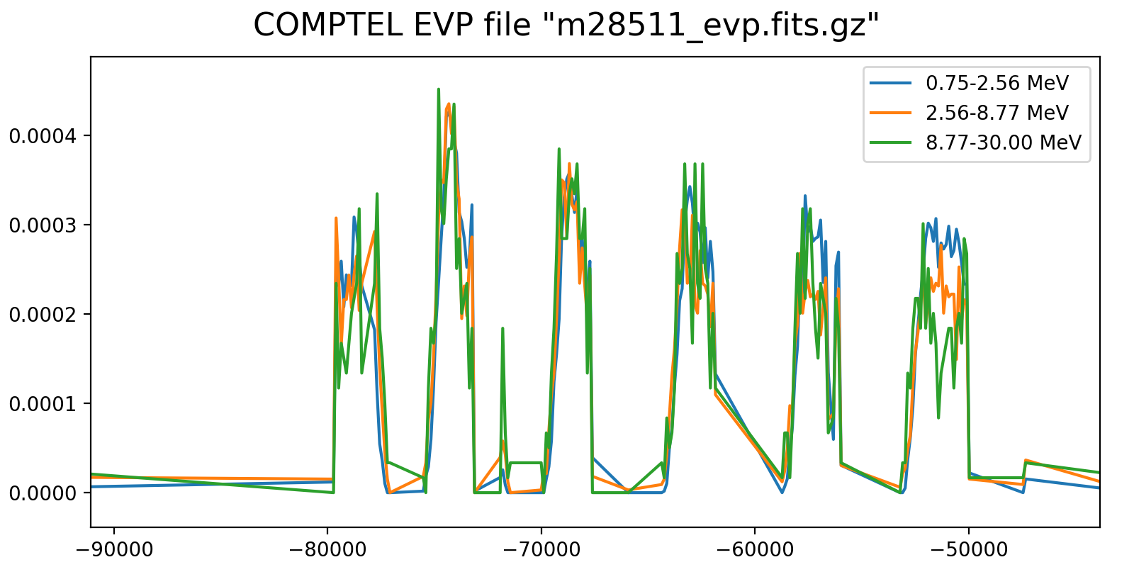
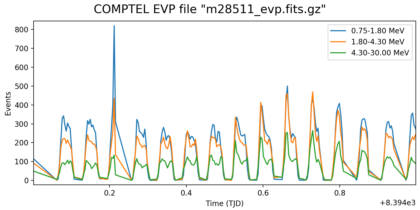
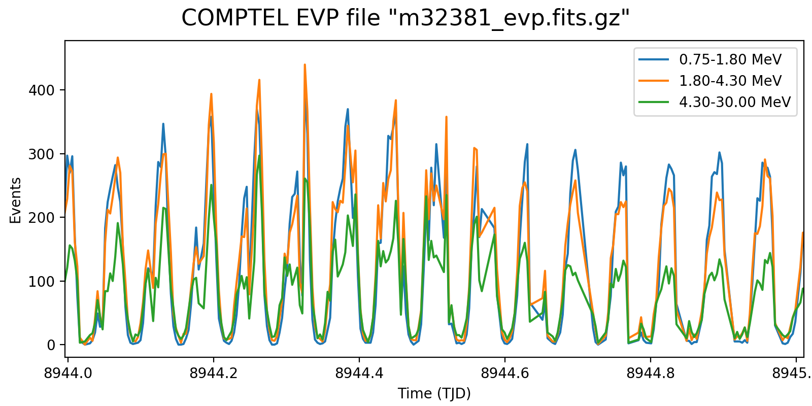
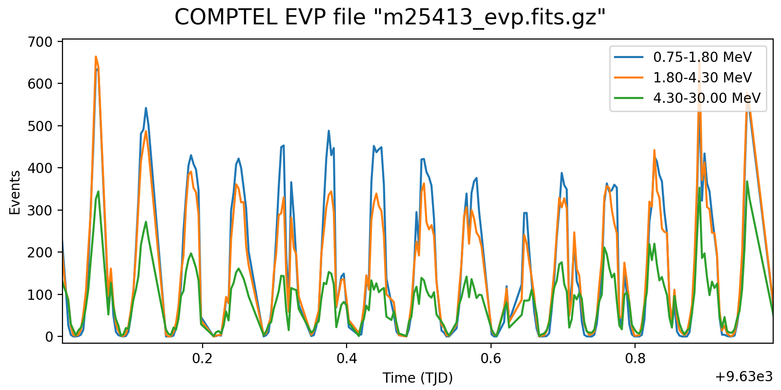
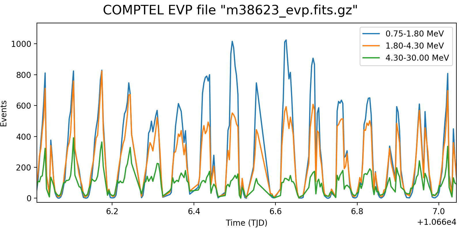
Following the reading of Georg’s PhD thesis it seems plausible to define representative energy ranges, for example 0.75-1.8 MeV, 1.8-4.3 MeV, and 4.3-30 MeV, and trace the temporal variation on a relatively short time scale for these energy ranges. Below the variations for one viewing period for each mission phase for a 5-minute rate computation, with a zoom into one day of data in the right column. Different rate trends are clearly visible in the three energy bands, minimum rates are typically 100 events, assuring a relative accuracy, while temporal trends and reasonably reproduced. I will now implement the DRW computation on this basis.
| 1.0 | 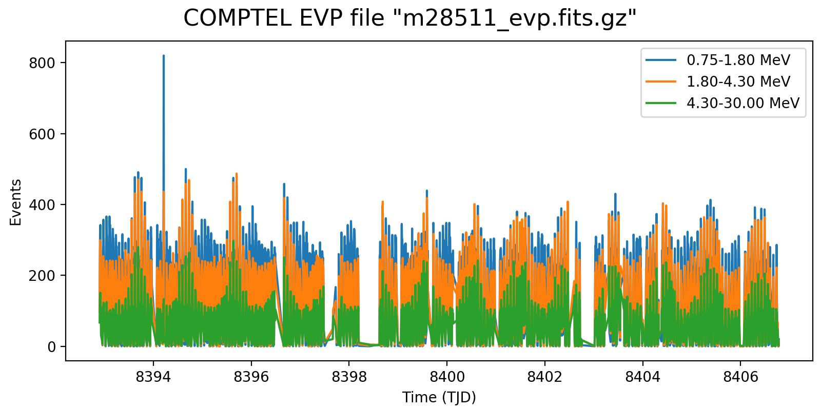 |
 |
| 201.0 | 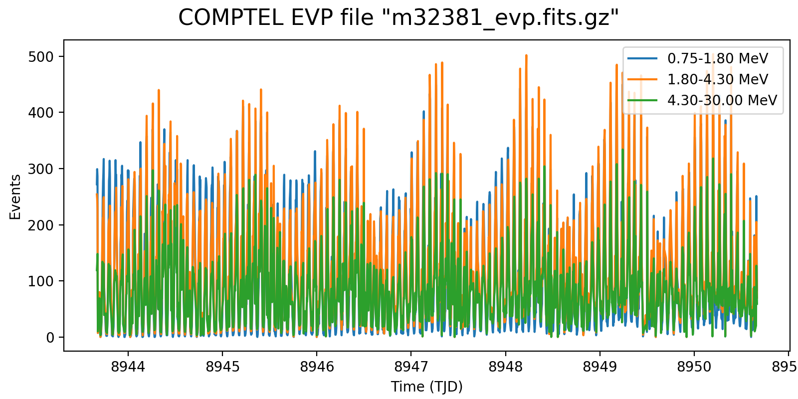 |
 |
| 301.0 |  |
 |
| 401.0 | 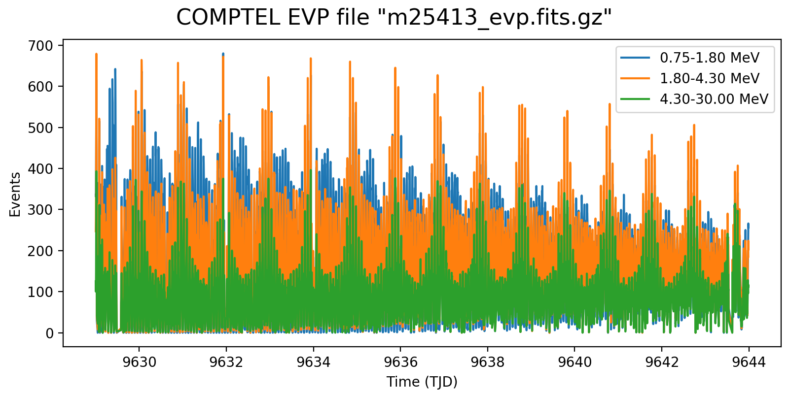 |
 |
| 501.0 | 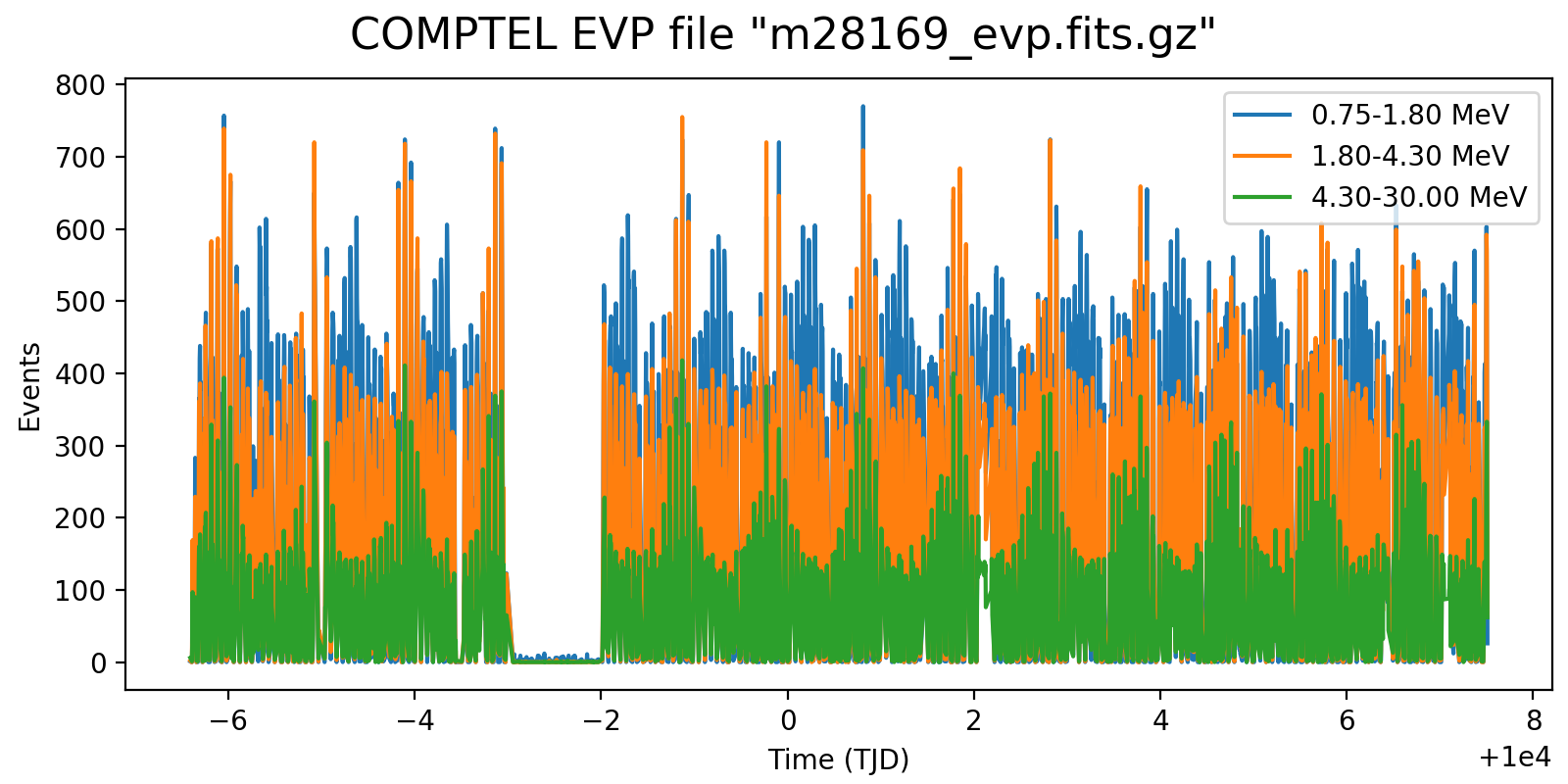 |
 |
| 625.0 |  |
 |
#7
Updated by Knödlseder Jürgen about 2 years ago
- File event-rate-vp625.0-5m-three-zoom.png added
- File event-rate-vp625.0-5m-three.png added
#8
Updated by Knödlseder Jürgen about 2 years ago
- % Done changed from 10 to 20
In the implementation of the computation there is an issue with computing time, since the calculation of the geometry factors is time consuming. Since the same geometry factors are needed for all energy bins, recomputation would be a huge waste of computing power.
One option would be to add a cache of the geometry values, yet this cache would consume quite some memory. With typically 60000 used superpackets and a binning of 80°x80° in Chi and Psi, about 3 GB of memory would be needed to cache the geometry values. This is huge, but the advantage would be that cached data, even from the DRG computation, could be reused as often as required. If a single class instance would be used to compute the DRG and then the DRW datacubes, geometry values would just be computed once.
An alternative option would be to implement a GCOMDris class that is a container class for GCOMDri instances, and that would implement the GCOMDris::compute_drw() method to compute efficiently the DRWs for all energy bins. This would not reused the geometry values from the DRG computation, hence increasing the overall computing time of the comobsbin script, which however, would not depend on the number of energy bins used. Setting different energy bins for an already viewing period would anyway not recompute the DRG, hence recomputation of the geometry values would be needed in any case. This is probably the better option as it avoids the handling of a large computation cache. And the container class could also be used to compute multiple DREs in one go, avoid the repeated looping over the superpackets and event lists. The drawback is, however, that there would be no control over already existing data sets, hence this would need to be handled when the GCOMDris container is setup, so that only non-existing energy bins would be added for computation.
A possible code thread in comobsbin would then look like
# Generate one DRW for each energy boundary
for i in range(ebounds.size()):

    # Set DRW filename
    drwname = '%s/%s%s_dre%s_%6.6d-%6.6dkeV.fits' % \
               (self['outfolder'].string(), obs.id(), dri_prefix, self._drw_suffix,
                ebounds.emin(i).keV(), ebounds.emax(i).keV())
    drwfile = gammalib.GFilename(drwname)

    # Set DRW filename in global data store
    drwname_global = '%s/%s%s_dre%s_%6.6d-%6.6dkeV.fits' % \
                      (self._global_datastore, obs.id(), dri_prefix, self._drw_suffix,
                       ebounds.emin(i).keV(), ebounds.emax(i).keV())
    drwfile_global = gammalib.GFilename(drwname_global)

    # Write header
    self._log_header3(gammalib.NORMAL, 'Compute DRW for %.3f - %.3f MeV' % \
                              (ebounds.emin(i).MeV(), ebounds.emax(i).MeV()))

    # If DRW file exists in global datastore then do nothing
    if drwfile_global.exists():
        drwname = drwname_global
        self._log_value(gammalib.NORMAL, 'Global DRW file exists', drwfile_global.url())

    # If DRW file exists then do nothing
    elif drwfile.exists():
        self._log_value(gammalib.NORMAL, 'Local DRW file exists', drwfile.url())

    # ... otherwise append DRW to container
    else:

        # Set DRW energy range
        drw.ebounds(gammalib.GEbounds(ebounds.emin(i), ebounds.emax(i)))

        # Append DRW to container
        drws.append(drw)

        # Append filename to list
        drwfiles.append(drwfile)

# If there are DRW files to compute then compute and save them now
if len(drwfiles) > 0:

    # Compute DRWs
    drws.compute_drws(obs, self._select, self['zetamin'].real())

    # Save DRWs
    for i, drwfile in enumerate(drwfiles):

        # Save DRW
        drws[i].save(drwfile, True)

        # Log creation
        self._log_value(gammalib.NORMAL, 'Local DRW file created', drwfile.url())

        # Log DRW
        self._log_string(gammalib.NORMAL, str(drw))
#9
Updated by Knödlseder Jürgen about 2 years ago
- % Done changed from 20 to 30
While working on the implementation I added equality operators to the GSkyMap class so that the consistency of DRWs can be easily checked.
#10
Updated by Knödlseder Jürgen about 2 years ago
- File phibar-impact.png added
- File phibar-impact-eha.png added
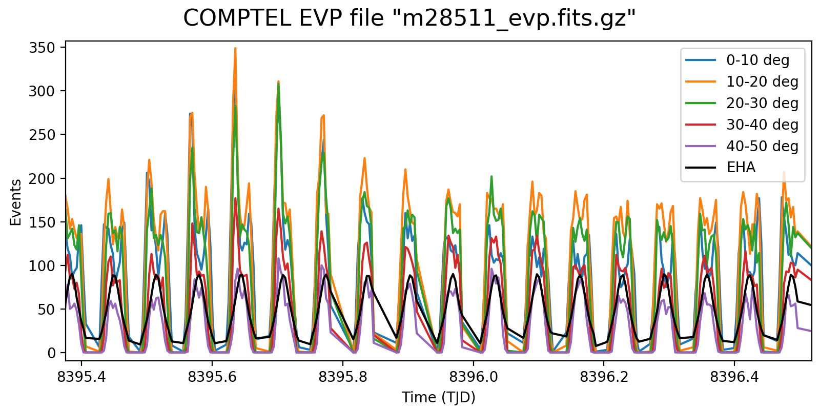
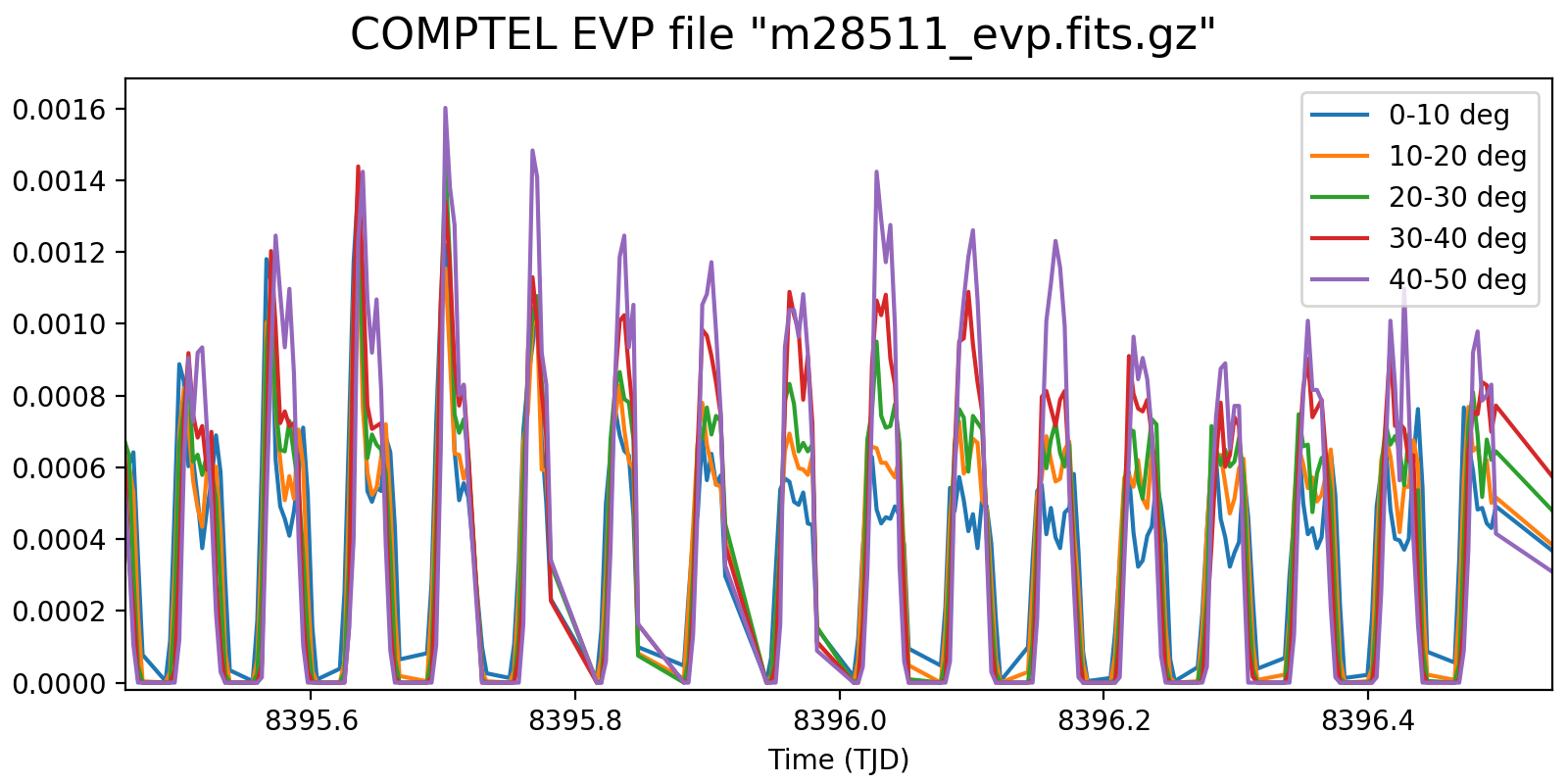
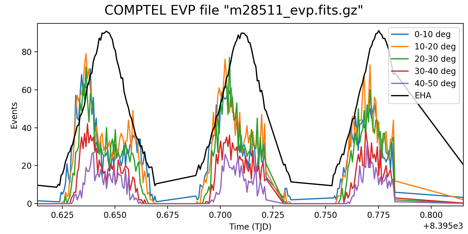
While playing with an initial implementation I figured out that there is a normalisation problem because the rates are in fact Phibar dependent. The total rate variations shown above encode both the variations in the background rates as well as the variations due to the Earth horizon cut. The issue is that the Earth-horizon-cut variations are Phibar dependent, resulting in rate variations that depend on Phibar.
This is illustrated in the figure below which shows the event rate as function of Phibar. In the left panel the event rates were normalised to match the variations in the various Phibar layers, in the right panel the absolute variations are shown. In addition, the black line shows the average Earth horizon angle of the events, illustrating the moments where the Earth is far from the field of view. Data are for VP 0001.0.
In the left plot there seem to be moments when there is not any Phibar dependence, while at other moments there is a string increase in the normalised rates with Phibar angle. Why is this so?
Interestingly, the right plot seems to indicate that there are dips in the event rates when the Earth horizon angle is larger, while there are peaks to the left and right in the event rate when the Earth horizon angle decreases. This is if the Earth was leaking into the field of view.
 |
 |
#11
Updated by Knödlseder Jürgen about 2 years ago
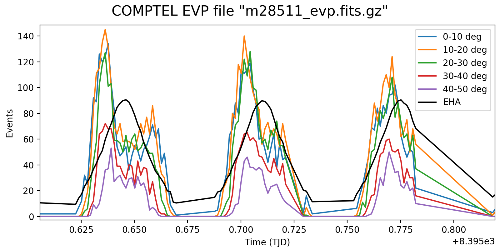
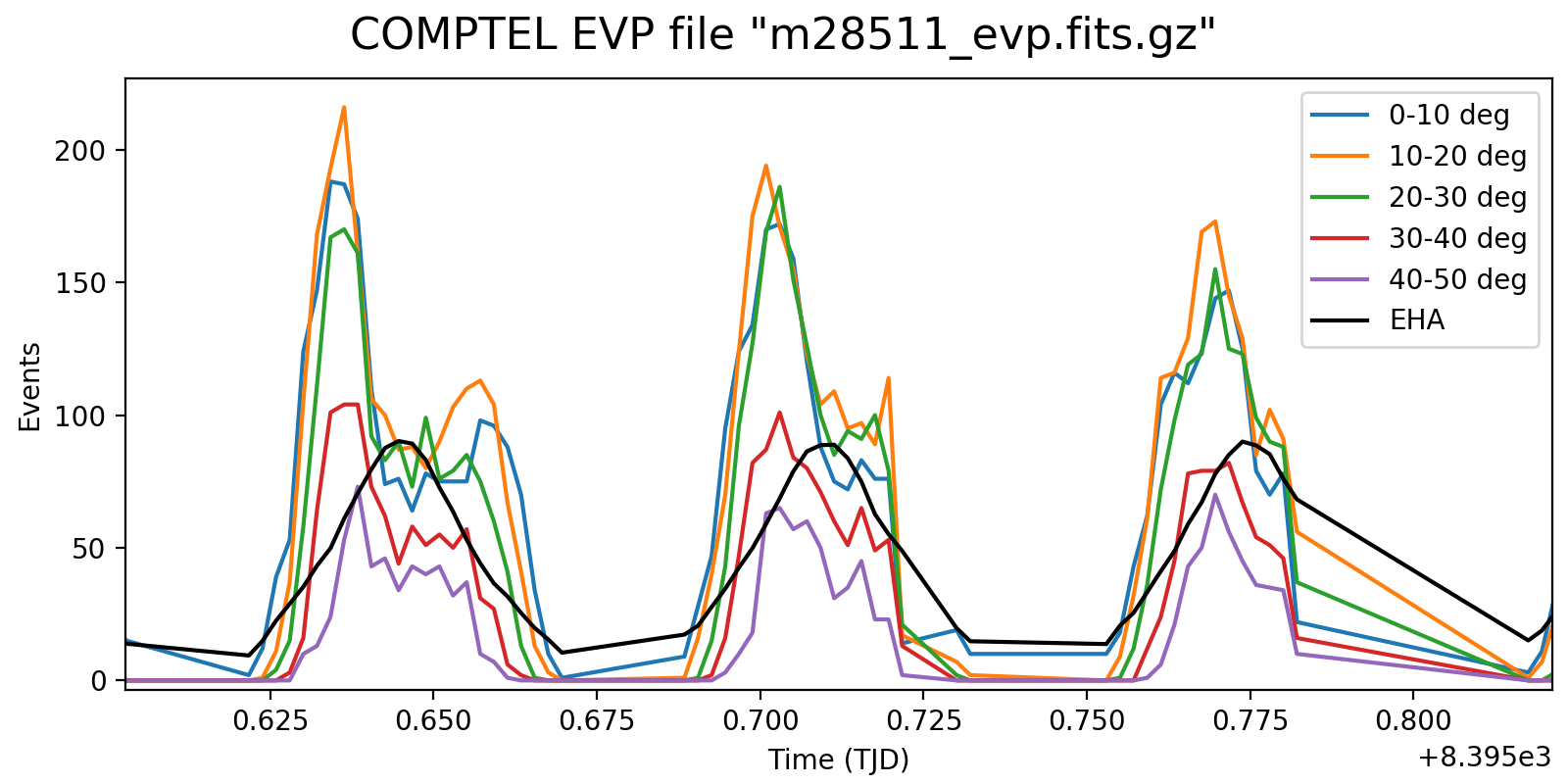
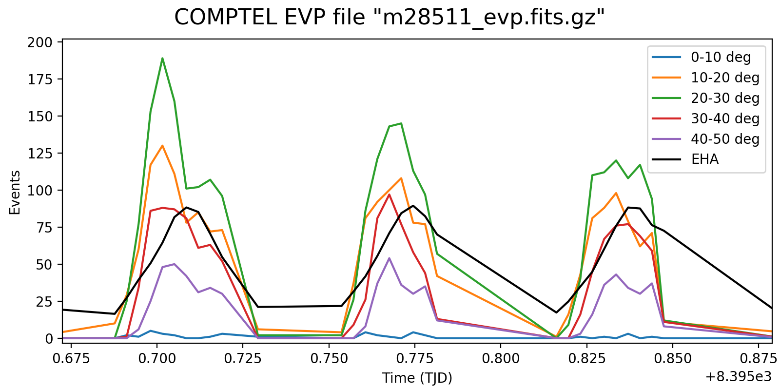
- File phibar-impact-eha-1min.png added
- File phibar-impact-eha-2min.png added
- File phibar-impact-eha-3min.png added
Below a detailed look into three orbits at different time resolutions of 1, 2 and 3 minutes. This reveals rate variations that are clearly Phibar dependent, which is no surprise as at larger Phibar angles the times when the Earth is not in the field of view decreases. While the left spikes at low Phibar angles can be explained by activation in the SAA (that is only visible in the low Phibar angles since the profiles “start earlier”), it is strange that the rates also rise towards the end of the orbit for Phibar < 20°.
 |
 |
 |
#12
Updated by Knödlseder Jürgen about 2 years ago
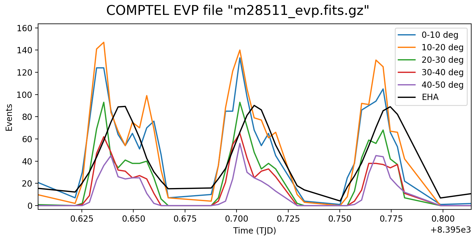
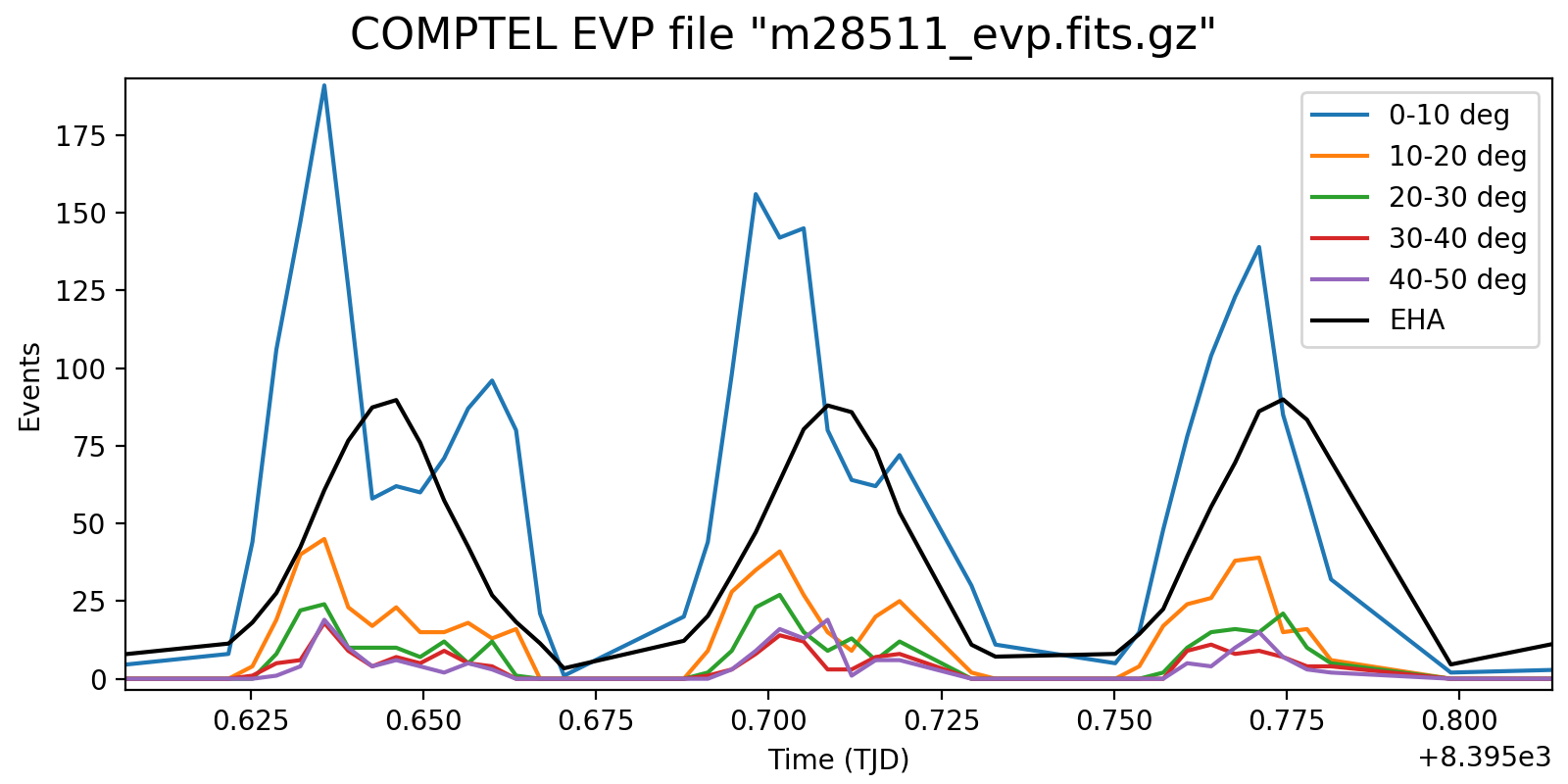
- File phibar-impact-high-5min.png added
- File phibar-impact-low-5min.png added
- File phibar-impact-mid-5min.png added
Below the rate variation for the three energy bands <1.8 MeV, 1.8-4.3 MeV and >4.3 MeV. The rate variation on the scale of an orbit seems to be strongly determined by the Phibar range.
#13
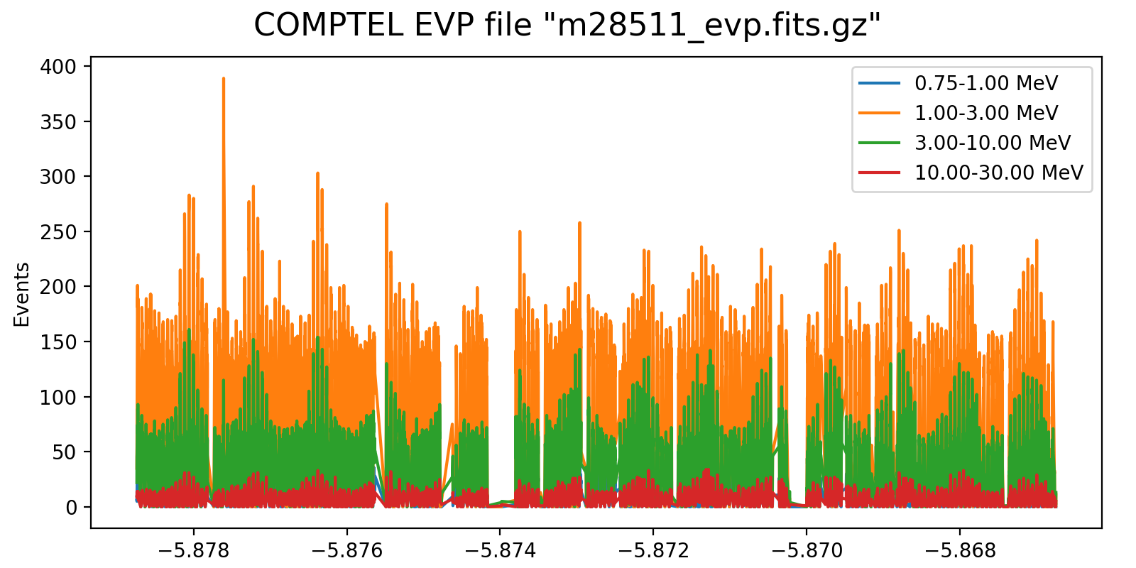
Updated by Knödlseder Jürgen about 2 years ago
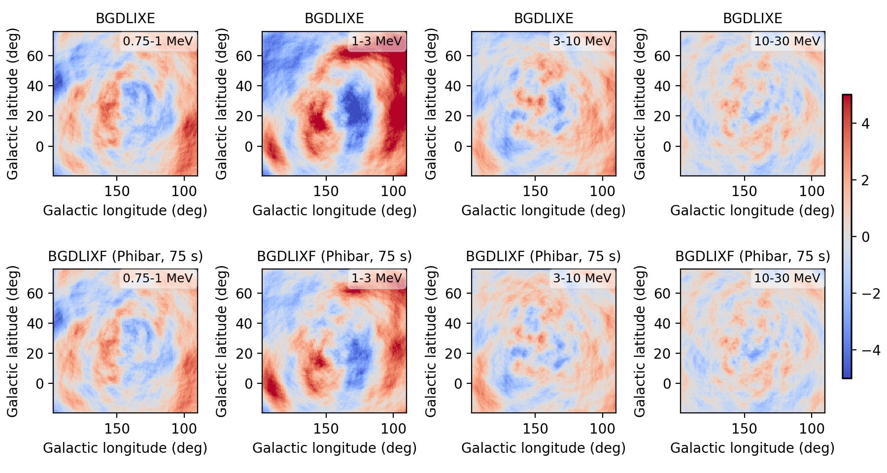
- File res_ehacorr_max10.png added
- File res_noehacorr.png added
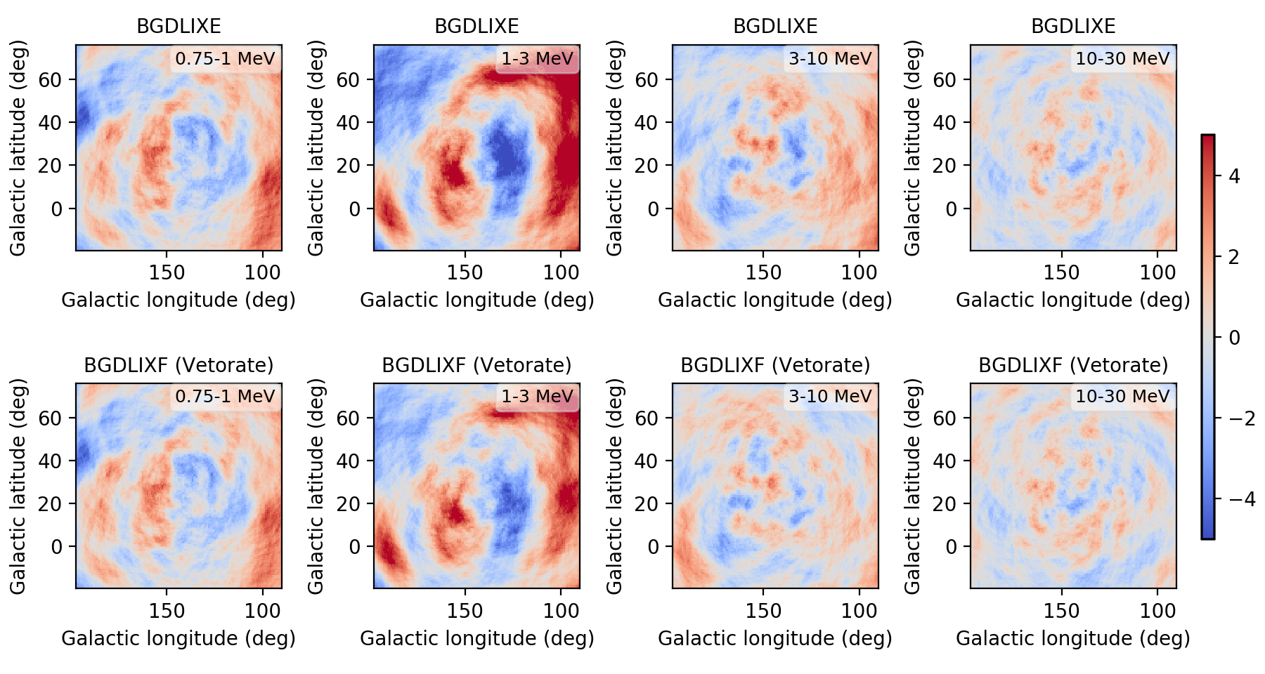
I implemented a Phibar-dependent weighting cube computation and tested the computation on viewing period 0518.5 which has the largest residuals. Below a comparison between the BGXLIXE method (top row) and the new BGXLIXF method (bottom row). For the left panel no correction for the Earth horizon cut was made, and the BGXLIXF background model actually is worse than the BGXLIXE model. Taking into account the correction of the Earth horizon cut leads to an improved BGXLIXF background model, with reduced residuals with respect to BGXLIXE. A timebin of 300 sec was used for the plots. Hence we are on the right track, emphasizing again that much of the variation shown above is due to the Earth horizon cut.
no EHACORR, 300 sec 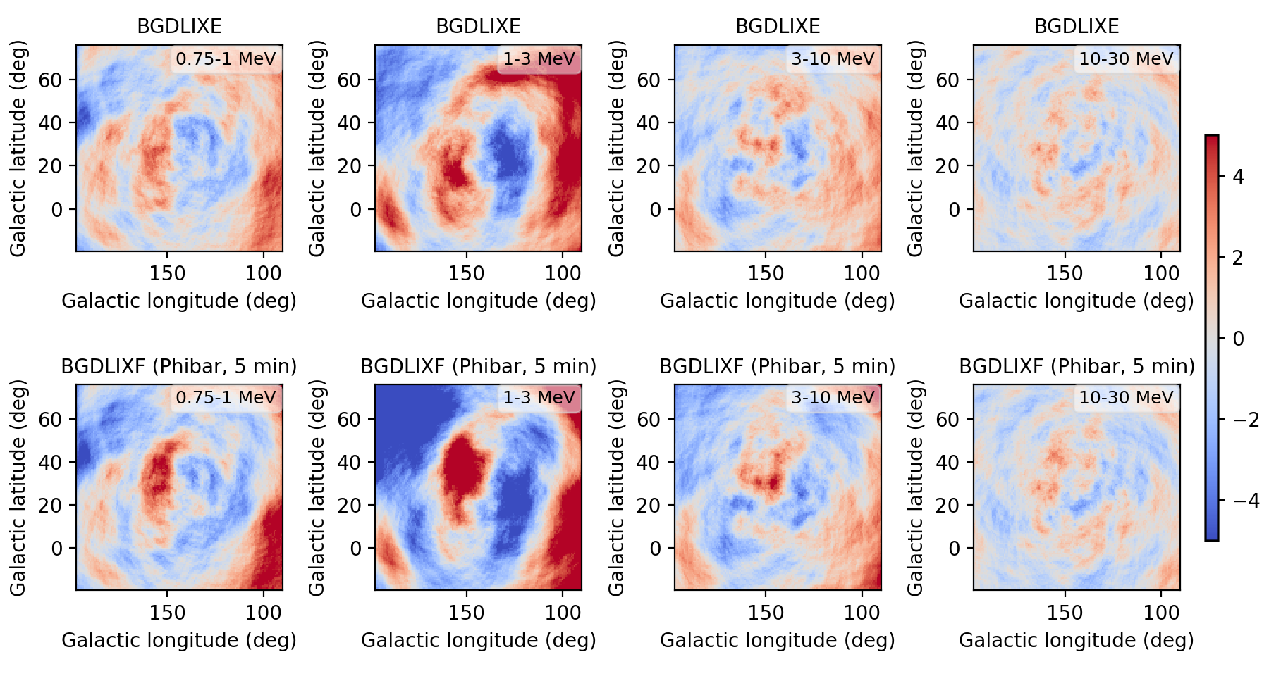 |
EHACORR<10, 300 sec 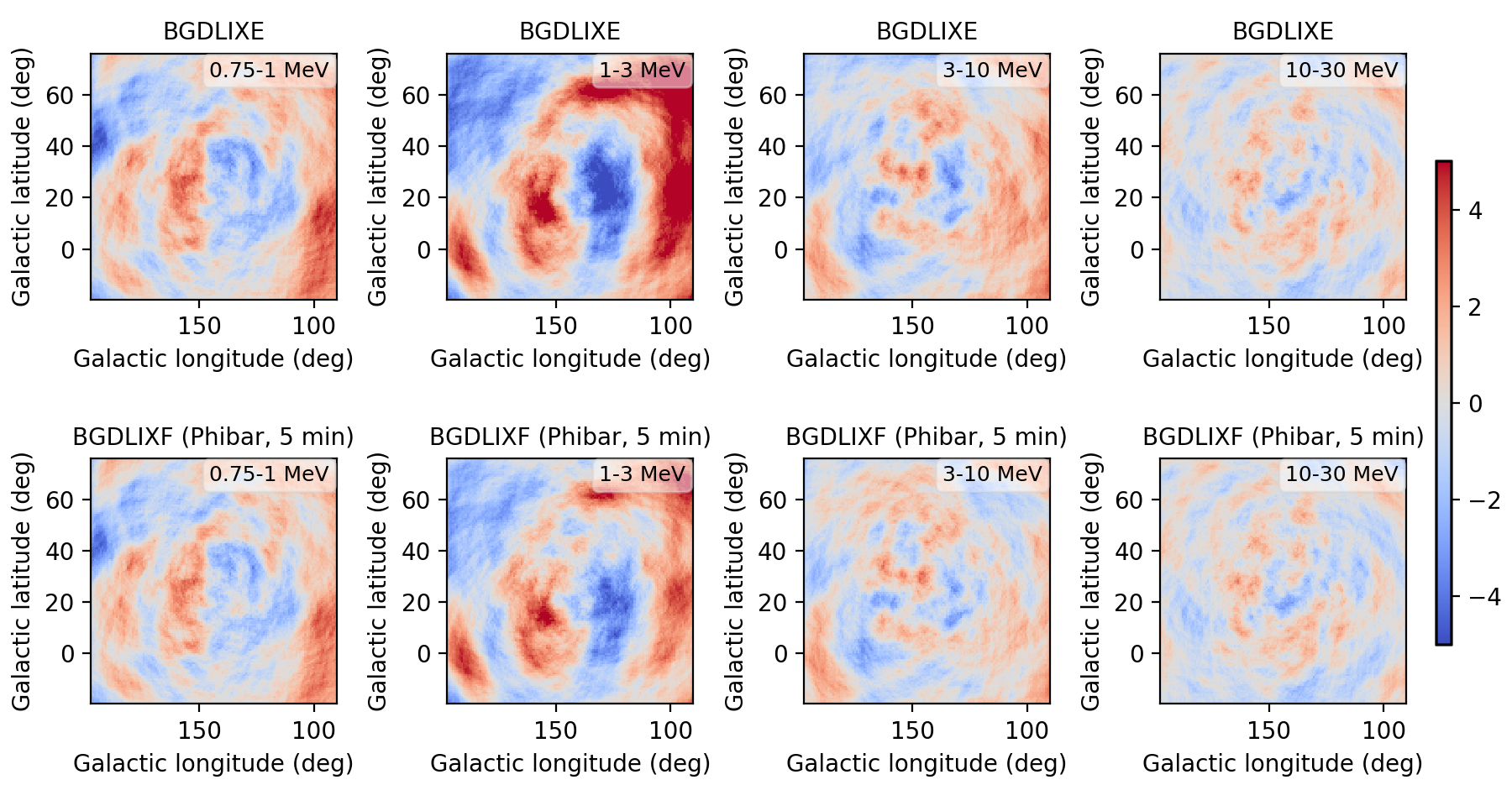 |
EHACORR<100, 300 sec 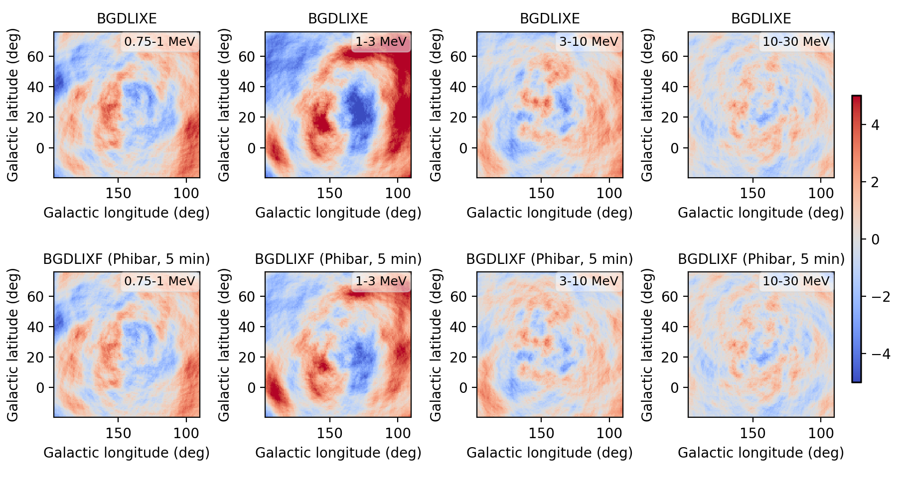 |
EHACORR<1000, 300 sec  |
EHACORR<10, 150 sec  |
EHACORR<10, 75 sec  |
Below the residual range in Gaussian sigma in a number of runs:
| Configuration | 0.75-1 MeV | 1-3 MeV | 3-10 MeV | 10-30 MeV |
| BGDLIXE | -5.23 - 5.02 | -6.94 - 7.58 | -4.22 - 4.03 | -3.35 - 3.44 |
| BGDLIXF, no EHACORR, 300 sec | -5.96 - 6.28 | -8.37 - 14.81 | -4.67 - 6.67 | -3.54 - 3.42 |
| BGDLIXF, EHACORR<10, 300 sec | -4.75 - 4.35 | -5.14 - 5.91 | -3.55 - 3.67 | -3.38 - 3.46 |
| BGDLIXF, EHACORR<100, 300 sec | -4.74 - 4.38 | -4.78 - 6.38 | -3.57 - 3.51 | -3.43 - 3.41 |
| BGDLIXF, EHACORR<1000, 300 sec | -4.74 - 4.38 | -4.75 - 6.37 | -3.57 - 3.51 | -3.43 - 3.41 |
| BGDLIXF, EHACORR<10, 75 sec | -4.64 - 4.31 | -4.93 - 6.14 | -3.58 - 3.55 | -3.48 - 3.30 |
| BGDLIXF, EHACORR<10, 150 sec | -4.67 - 4.34 | -4.90 - 6.16 | -3.55 - 3.57 | -3.43 - 3.36 |
| BGDLIXF, EHACORR<10, 300 sec | -4.75 - 4.35 | -5.14 - 5.91 | -3.55 - 3.67 | -3.38 - 3.46 |
| BGDLIXF, EHACORR<10, 600 sec | -4.84 - 4.50 | -4.96 - 7.14 | -3.65 - 3.79 | -3.45 - 3.49 |
| BGDLIXF, EHACORR<10, 1200 sec | -5.03 - 4.68 | -6.31 - 8.74 | -4.81 - 4.55 | -3.44 - 3.65 |
#14
Updated by Knödlseder Jürgen about 2 years ago
- File res_ehacorr_max100.png added
#15
Updated by Knödlseder Jürgen about 2 years ago
- File res_ehacorr_max1000.png added
#16
Updated by Knödlseder Jürgen about 2 years ago
- File res_ehacorr_max10_75sec.png added
- File res_ehacorr_max10_150sec.png added
#17
Updated by Knödlseder Jürgen almost 2 years ago
- File logl-profiles-vp0518.5.png added
- % Done changed from 30 to 40
I started the implementation of an alternative approach that should be more accurate and allow the implementation of an energy dependence of the rate variations, yet that requires using Housekeeping data (HKD data structures) and that requires two evaluate two times the geometry function for each superpacket.
The basic idea follows the observation of Weidenspointner et al. (1999) that the event rate variation has a prompt component and some components related to build-up of activation with longer time scales. While above 4.3 MeV only the prompt component is observed, build-up of activation with longer time scales is seen below that energy.
Following the investigations of Weidenspointner et al. (1999), we assume that the prompt component is traced by the Veto rate, and specifically the rate in the 2nd veto dome, dubbed SCV2M, while the build-up of activation can be modelled by a constant rate at the time scale of a viewing period (typically two weeks). The background event rate is thus given by
rate(t,phibar) = n(phibar,iebin) * [ f_prompt * vetorate(t,phibar) + (1 - f_prompt) * constrate(t,phibar) ]
where
n(phibar,iebin) = norm * sum_t N(t,phibar,iebin) / sum_t [ f_prompt * vetorate(t,phibar) + (1 - f_prompt) * constrate(t,phibar) ]
is a phibar and energy normalisation constant that assures that the time-integrated background rate corresponds to the measured number of events for each phibar interval and energy bin, and
norm=1.0 is a scaling factor. Here, N(t,phibar,iebin) is the number of events for a given superpacket t, phibar interval and energy bin.
vetorate(t,phibar) and constrate(t,phibar) are the expected rate variations after taking into account any Earth horizon cut. The Earth horizon cut introduces in fact a time-variation of the event rate that in general differs in frequency, phase and amplitude from the time-variation introduced by the intrinsic background rate variation. The expected time variation of the Earth horizon cut can be computed by applying for a given superpacket the Earth horizon cut to the geometry function and computing that fraction of geometry that survives the cut with respect to the integrated geometry function. Note that the geometry function needs to be multiplied by the solid angle of the spatial bins to turn the probability into an expected event rate. The resulting fraction is stored in an array
ehacutcorr(t,phibar)and the Veto rate and constant rate arrays are computed using
vetorate(t,phibar) = n_veto * veto(t) * ehacutcorr(t,phibar)and
constrate(t,phibar) = n_const * 1 * ehacutcorr(t,phibar)where
n_veto and n_const are normalisation constants that assure that the time integrated rates equal to one:n_veto = 1 / sum_t veto(t)and
n_const = 1 / sum_t 1
f_prompt is then the fraction of the background rate that is related to prompt background, and is comprised with [0,1].
I implemented GCOMHkd and GCOMHkds methods to manage COMPTEL housekeeping data and extended the comgendb script to attach the housekeeping files to the observation definition XML file. There is in fact one housekeeping file per day, and it turned out that in the HEASARC database there is only one corrupt HKD file:
2023-03-22T09:06:45: +=======================+
2023-03-22T09:06:45: | Get list of HKD files |
2023-03-22T09:06:45: +=======================+
2023-03-22T09:07:20: *** Corrupt HKD file "$COMDATA/phase02/vp0232_5/m22444_hkd.fits" encountered. Set HKD quality to -200.
2023-03-22T09:07:20: *** HKD file "$COMDATA/phase02/vp0232_5/m22444_hkd.fits" has quality -200. Skip file.
I implemented a logic that excluded the corresponding OAD file from the database, so that for each available OAD file there is a corresponding HKD file in the database.
I then implemented GCOMDris::compute_drws_vetorate method that for the moment computes some required arrays and stores them into a FITS file for diagnosis. Specifically, the method calls the method GCOMDris::setup_wrk_vetorate that sets-up working arrays holding the following data:
m_wrk_counts     - N(t,phibar,iebin)
m_wrk_ehacutcorr - ehacutcorr(t,phibar)
m_wrk_vetorate   - veto(t)
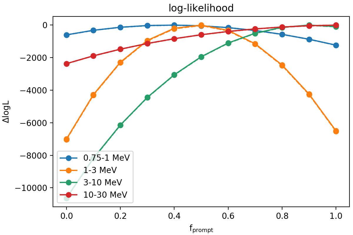
I implemented some Python code to read these FITS files and to determine the best fitting f_prompt parameter for the standard energy bands using a log-likelihood computation. As example I used viewing period 518.5 since it has the largest residuals using the traditional BGDLIXE method. Below is a figure with the log-likelihood profiles for the four standard energy bands. For the 3-10 MeV and 10-30 MeV energy bands a f_prompt ~ 1 is obtained, while for lower energies f_prompt ~ 0.4-0.5, indicating long-lasting background components. This behaviour is exactly as expected based on the work of Weidenspointner et al. (1999), who found that above 4.3 MeV the background only has a prompt component. This illustrates that determining the background component mix from a log-likelihood fit to the time variation of the data actually works.

Note that the profiles where determines using norm=1 (solid lines), norm=0.99 (dotted lines) and norm=1.01 (dashed lines). The dotted and dashed lines are barely visible, yet they fall below the solid line, indicating that norm=1 is the maximum likelihood choice.
#18
Updated by Knödlseder Jürgen almost 2 years ago
- File fit_eventrates.py added
I also implemented a maximum likelihood fitting approach. Here the results for the 4 standard energy bands and viewing period 518.5. The f_prompt parameter was initialised to 0.5:
0.75-1 MeV ..: 206443.345 (0.38826 +/- 0.00592), 8 iterations
1-3 MeV .....: 852066.374 (0.48701 +/- 0.00219), 6 iterations
3-10 MeV ....: 525169.460 (0.90976 +/- 0.00334), 11 iterations
10-30 MeV ...: 136617.278 (1.00000 +/- 0.00815), 5 iterations
The fitting nicely confirms the log-likelihood profiles shown above.
I also tried for the 1-3 MeV energy band various initial values for f_prompt. The fit always converges to the same result, yet the required number of iterations may differ:
Init=0.0: 852066.373 (0.48680 +/- 0.00000), 4 iterations
Init=0.1: 852066.392 (0.48595 +/- 0.00000), 60 iterations
Init=0.2: 852066.380 (0.48628 +/- 0.00000), 29 iterations
Init=0.3: 852066.376 (0.48646 +/- 0.00131), 18 iterations
Init=0.4: 852066.374 (0.48660 +/- 0.00175), 12 iterations
Init=0.5: 852066.374 (0.48701 +/- 0.00219), 6 iterations
Init=0.6: 852066.374 (0.48697 +/- 0.00263), 7 iterations
Init=0.7: 852066.374 (0.48693 +/- 0.00306), 6 iterations
Init=0.8: 852066.373 (0.48687 +/- 0.00350), 5 iterations
Init=0.9: 852066.373 (0.48682 +/- 0.00394), 4 iterations
Init=1.0: 852066.373 (0.48680 +/- 0.00438), 3 iterations
#19
Updated by Knödlseder Jürgen almost 2 years ago
- File res_binned_vp0518.5_bgdlixf-vetorate.png added
- % Done changed from 40 to 50
Generating now a residual map and comparing to the previous results gives the following. The residuals are better than those of the BGDLIXE model, yet slight worse than those for the Phibar-BGDLIXF model, which is disappointing. I had hoped that the residuals will become better. Note that there is some slight improvement for the higher energies, yet at lower energies the model is slightly worse. I probably should inspect the count rate variation and see whether I can spot any issue. Maybe there are background rate variations with time scales shorter than two weeks involved, which could explain why Phibar-BGDLIXF is slightly better.
| Configuration | 0.75-1 MeV | 1-3 MeV | 3-10 MeV | 10-30 MeV |
| BGDLIXE | -5.23 - 5.02 | -6.94 - 7.58 | -4.22 - 4.03 | -3.35 - 3.44 |
| BGDLIXF, EHACORR<10, 300 sec | -4.75 - 4.35 | -5.14 - 5.91 | -3.55 - 3.67 | -3.38 - 3.46 |
| BGDLIXF, VETORATE | -4.89 - 4.65 | -5.22 - 6.40 | -3.43 - 3.67 | -3.20 - 3.34 |

#20
Updated by Knödlseder Jürgen almost 2 years ago
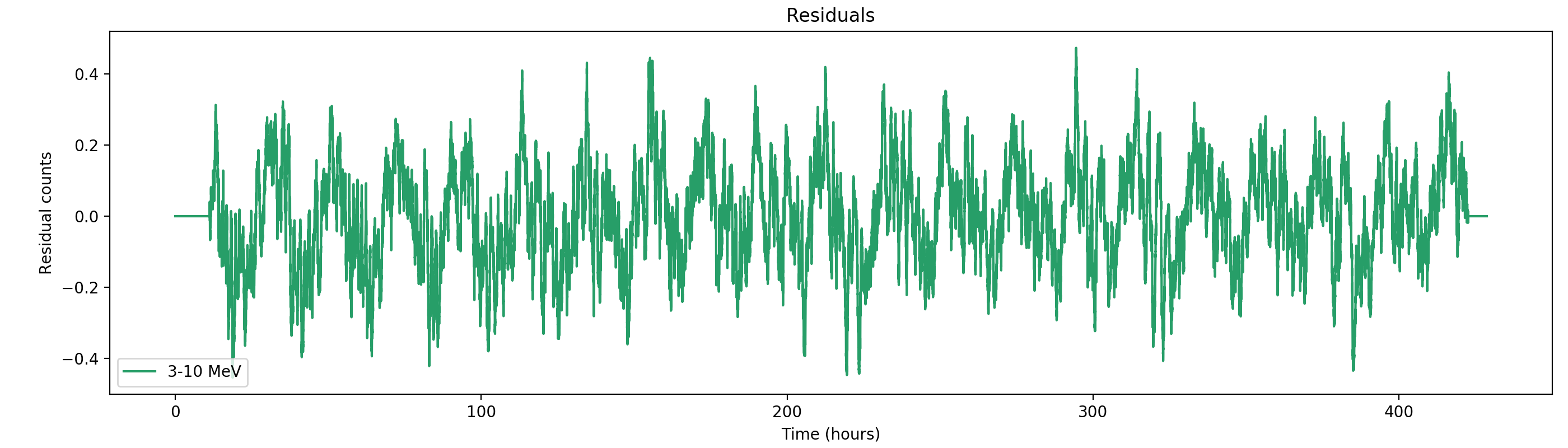
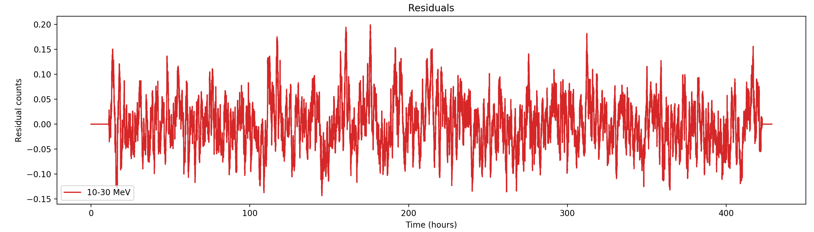
- File residuals0.png added
- File residuals1.png added
- File residuals2.png added
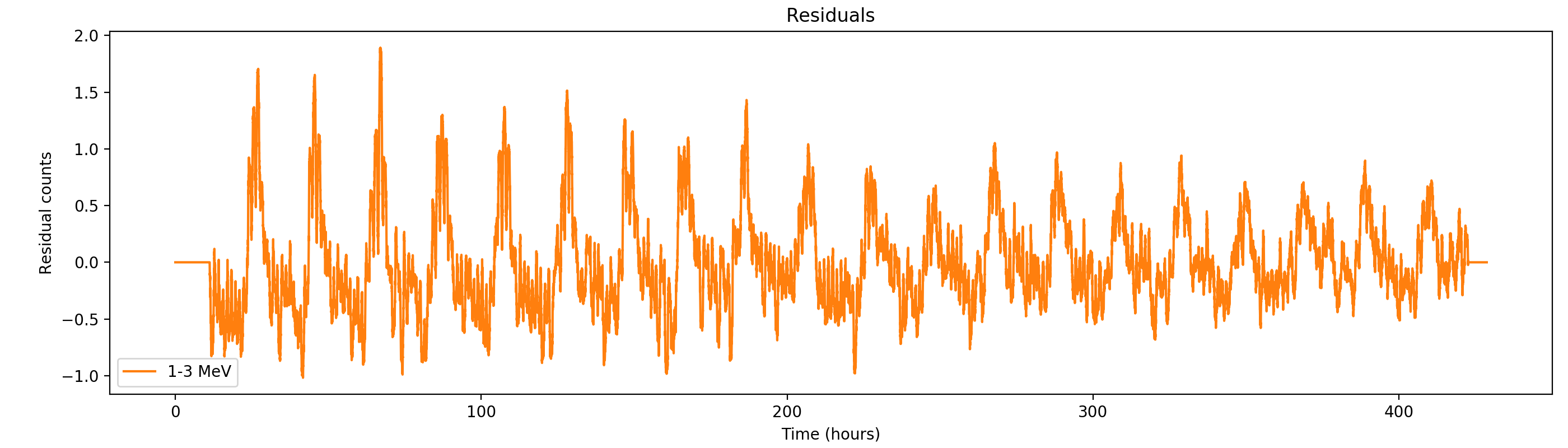
- File residuals3.png added
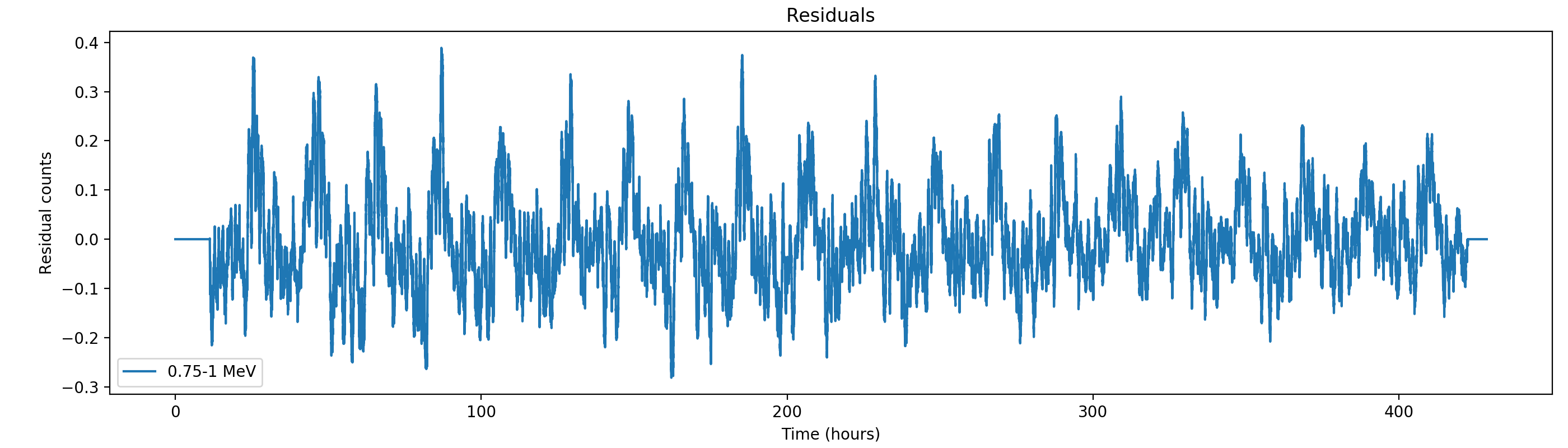
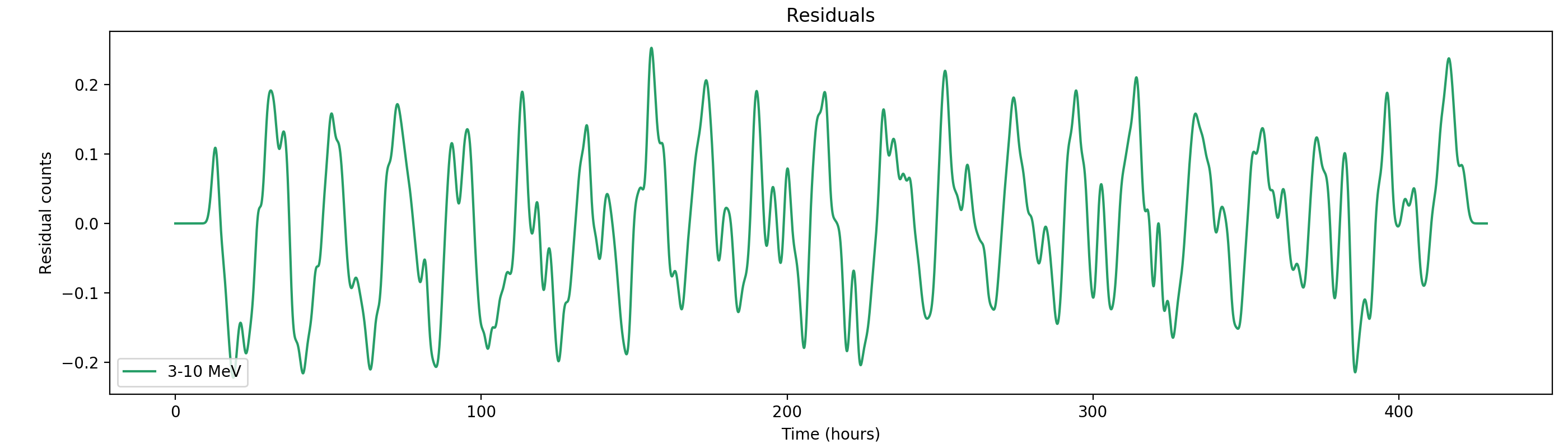
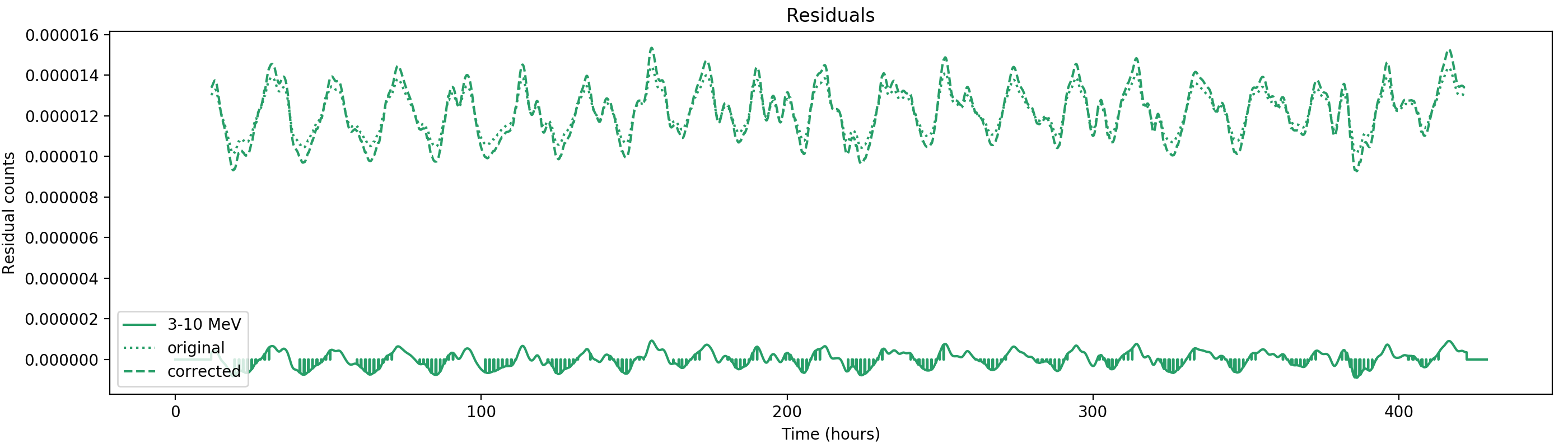
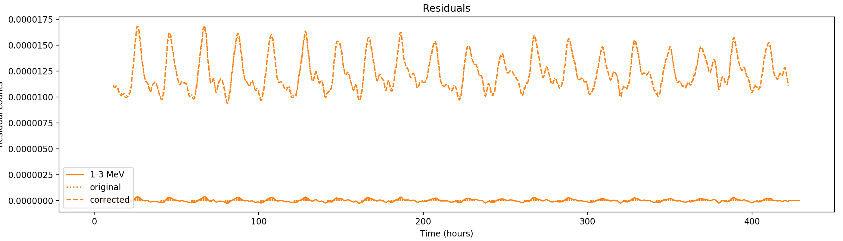
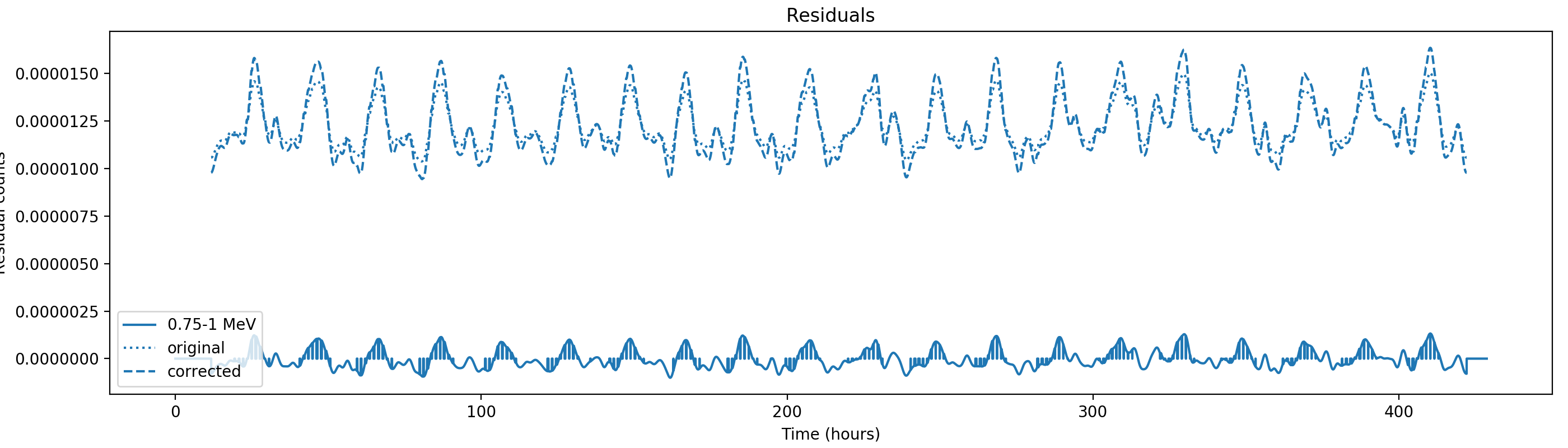
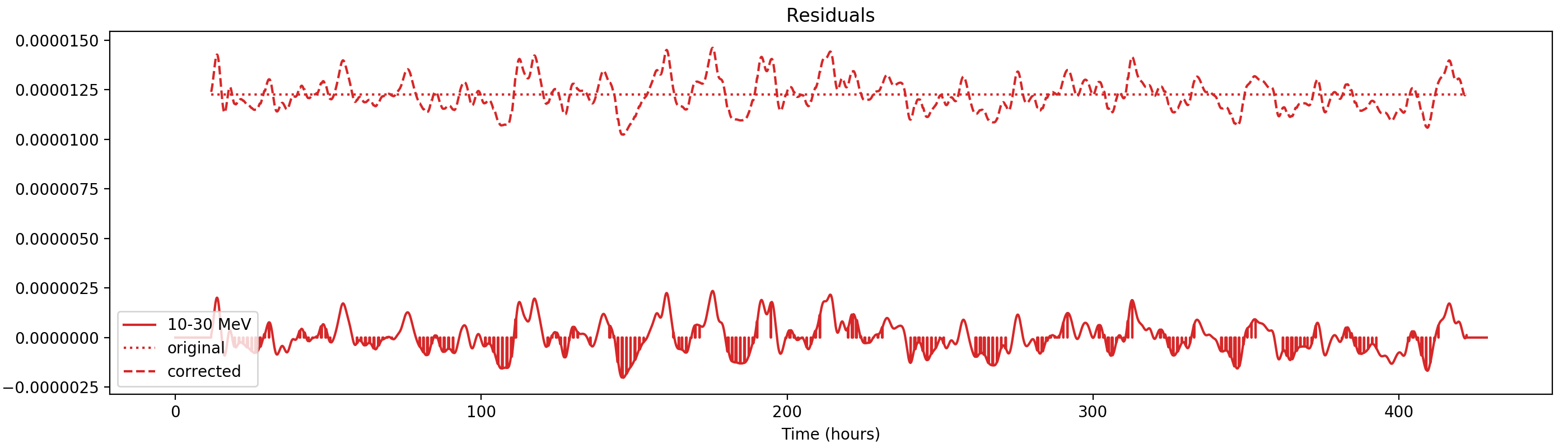
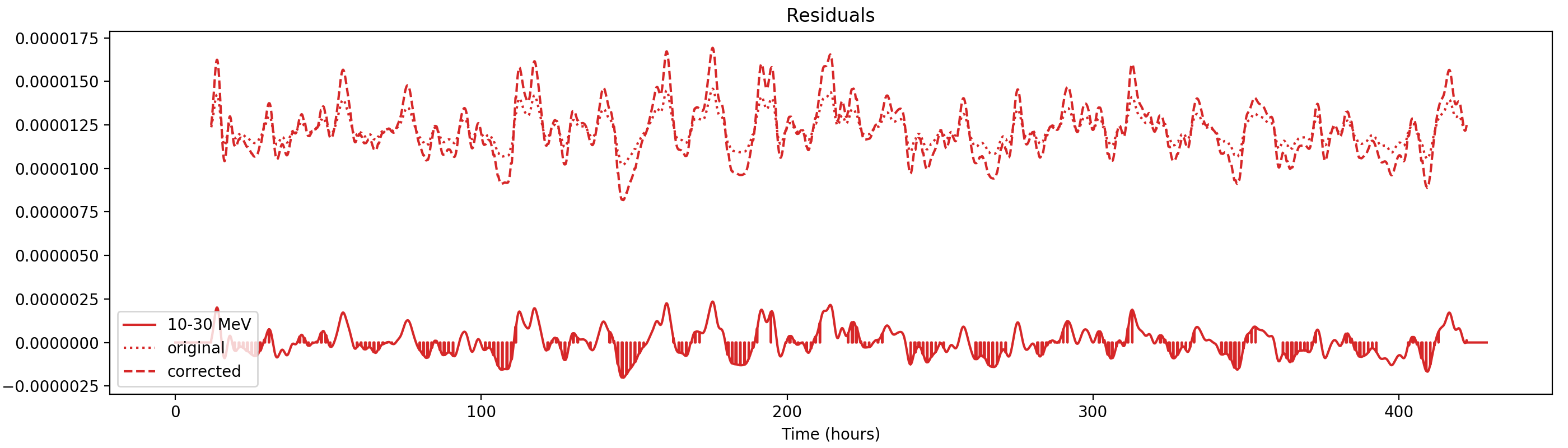
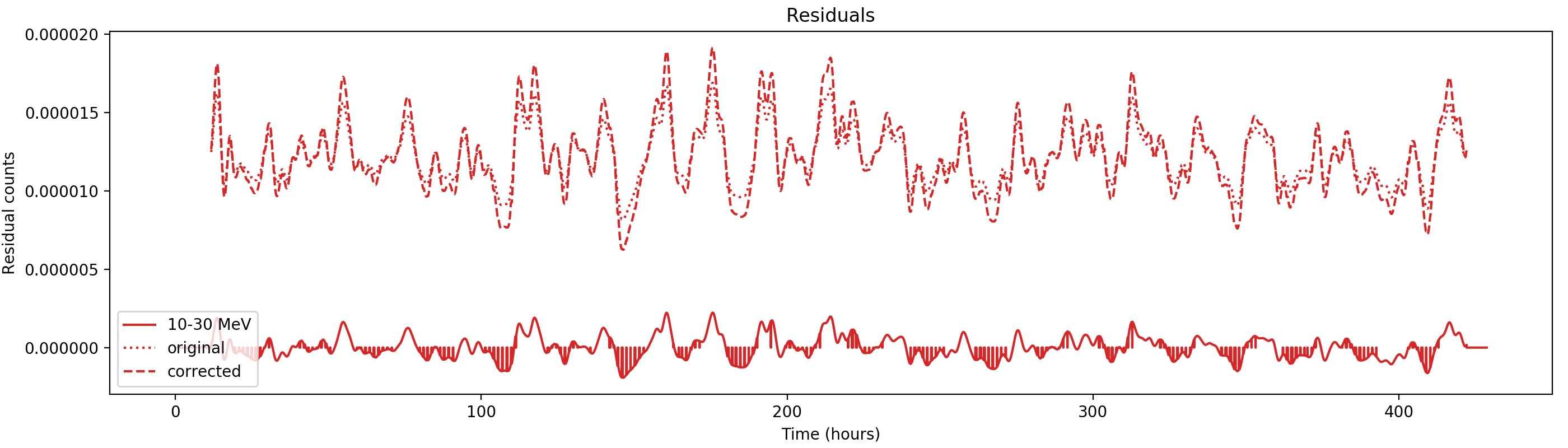
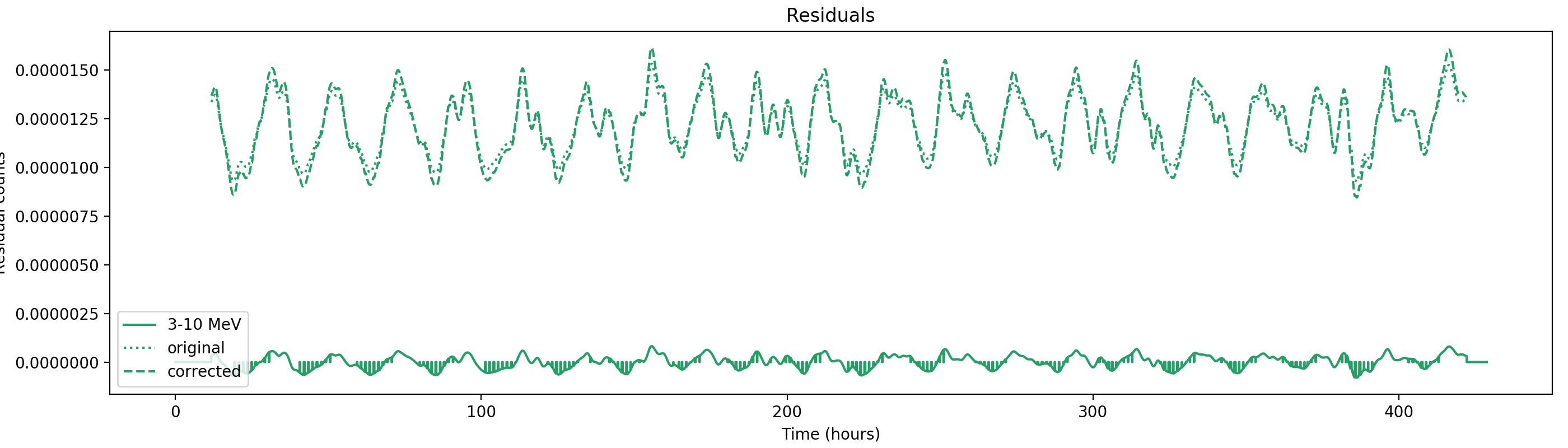
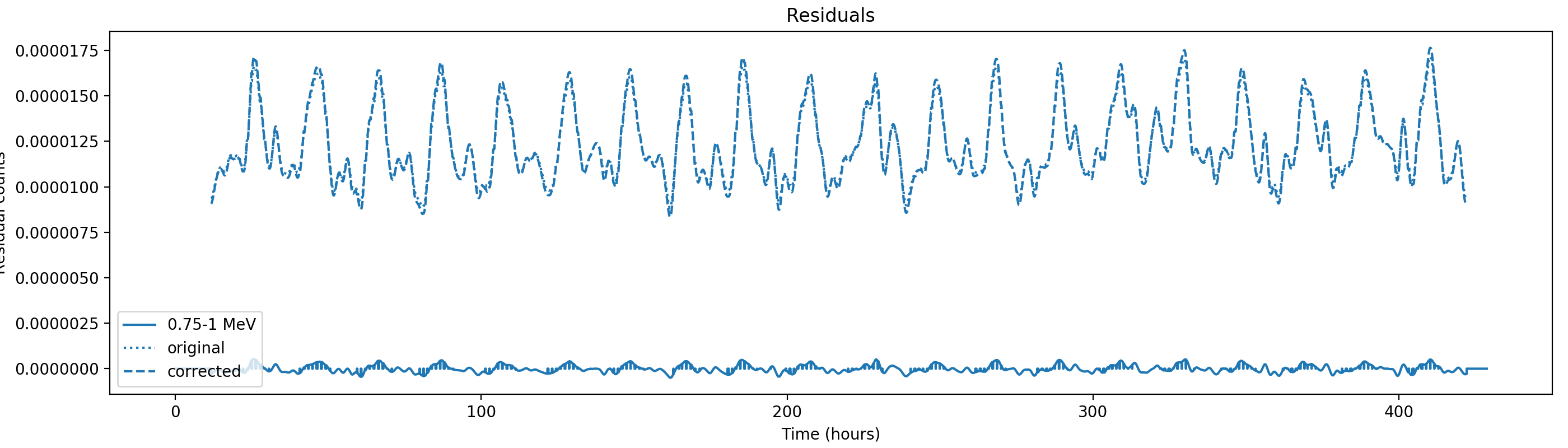
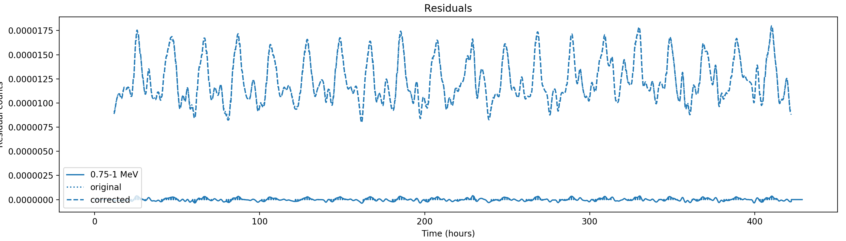
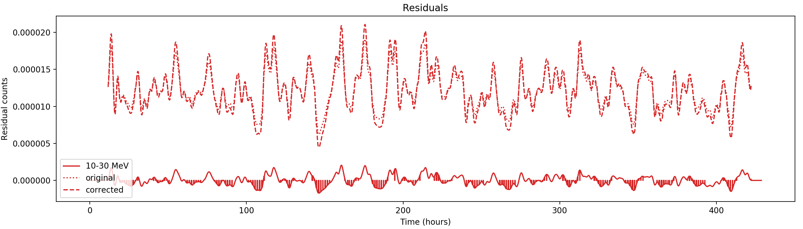
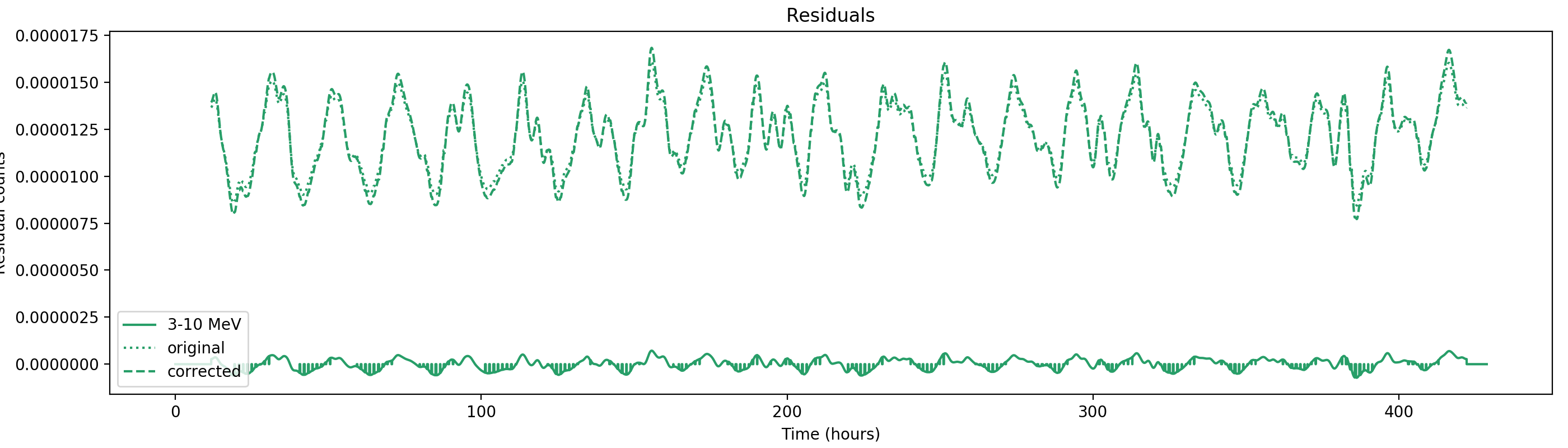
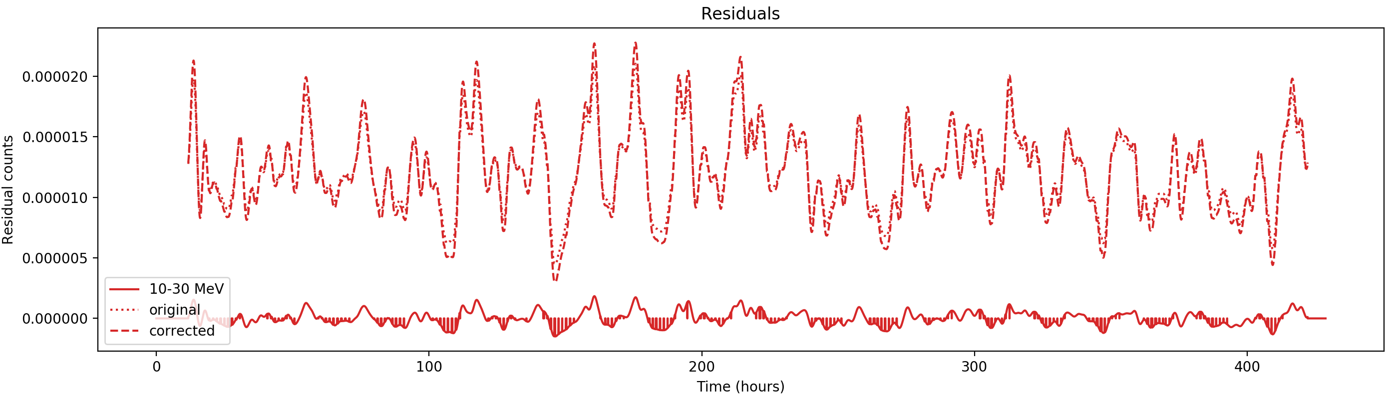
Here the residual counts for all four standard energy bands, smoothed with a boxcar average with a width of 220 superpackets, corresponding to about one hour. There is a clear period residual structure visible, in particular for the two lower energy bands, with a periodicity of about 21 hours. It looks like this periodicity may come from activation following SAA packages, which occur only at specific times during a day. In particular the 1-3 MeV residuals indicating an asymmetric shape of the residuals, with a sharp rise and a longer lasting decay.

#21
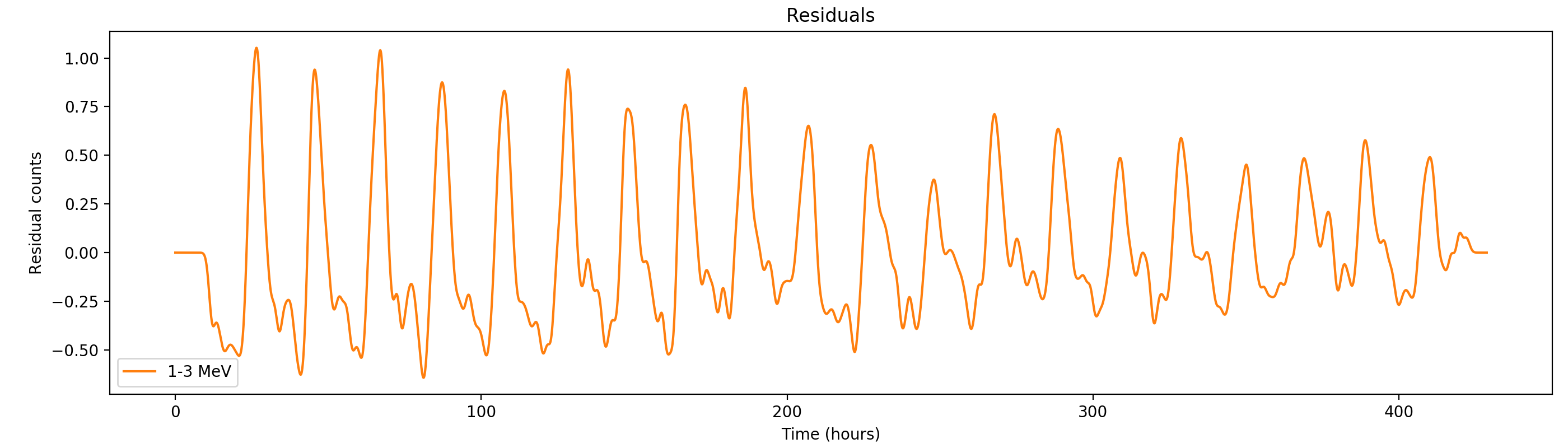
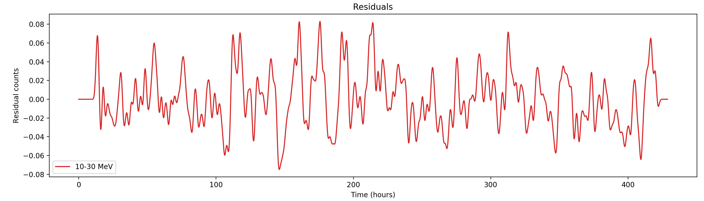
Updated by Knödlseder Jürgen almost 2 years ago
- File residuals0-gauss1h.png added
- File residuals1-gauss1h.png added
- File residuals2-gauss1h.png added
- File residuals3-gauss1h.png added
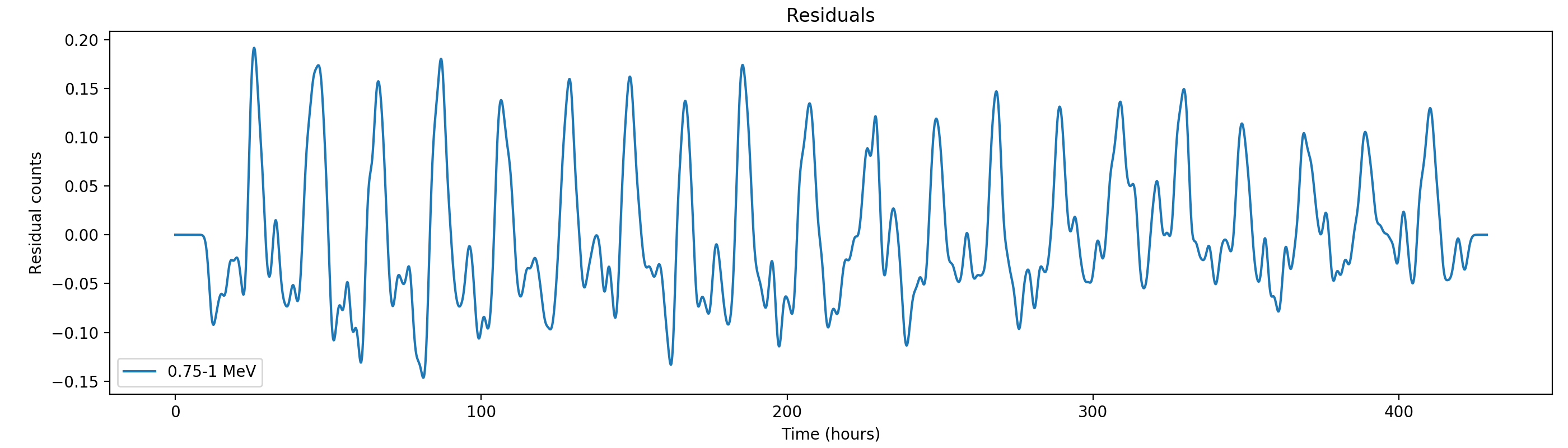
Here the same with a Gaussian smoothing kernel with sigma = 1 hour:


#22
Updated by Knödlseder Jürgen almost 2 years ago
- File corrected1-fc1-gauss1h-1st.png added
- File corrected1-fc1-gauss1h-2nd.png added
- File corrected1-fc1-gauss1h-3rd.png added
- File corrected1-fc1-gauss1h-4th.png added
- File corrected2-fc1-gauss1h-1st.png added
- File corrected2-fc1-gauss1h-2nd.png added
- File corrected2-fc1-gauss1h-3rd.png added
- File corrected1-fc1-gauss1h-5th.png added
- File corrected0-fc1-gauss1h-1st.png added
- File corrected0-fc1-gauss1h-2nd.png added
- % Done changed from 50 to 60
The above curves are after applying the Earth horizon cut correction, hence to correct the rates one has to “remove” the correction. The predicted number of residual counts res(t,phibar) is related to the “incident” residual rate (i.e. before applying the Earth horizon cut corrction) by
res_pred(t,phibar) = n(phibar) * ehacorrcut(t,phibar) * res(t)Summing over
phibar givesres_pred(t) = res(t) * sum_phibar n(phibar) * ehacorrcut(t,phibar)with
ehacorrcut(t) = sum_phibar n(phibar) * ehacorrcut(t,phibar)and
n(phibar) is the phibar-dependent normalisation factor. Hence the true residual rate res(t) is given byres(t) = res_pred(t) / ehacorrcut(t)
To avoid outliers due to small values of ehacorrcut(t) the smoothing operations needs to be applied to res_pred(t) and ehacorrcut(t), hence
res(t) = smooth[ res_pred(t) ] / smooth[ ehacorrcut(t) ]
It appeared that smoothing of ehacorrcut(t) led to spurious results at the beginning due to superpackets that were not used, hence to remove these spurious results I compressed the data by removing unused superpackets and applying the FFT for smoothing on the compressed results. This is not fully clean since it does not conserve the time scales. Instead, a brute force Gaussian convolution should be implemented that respects missing data.
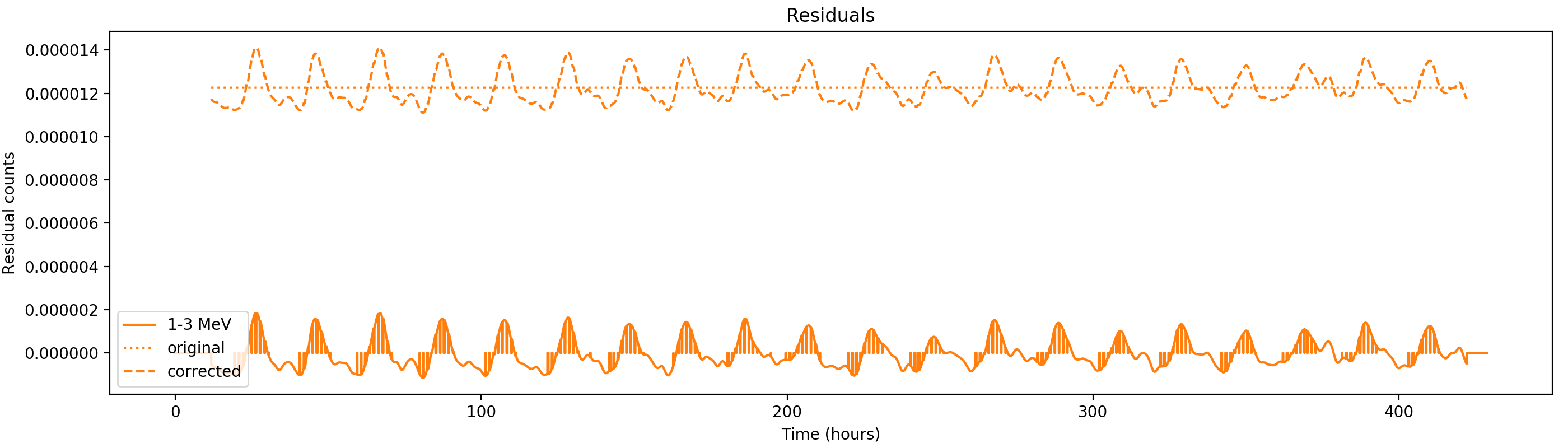
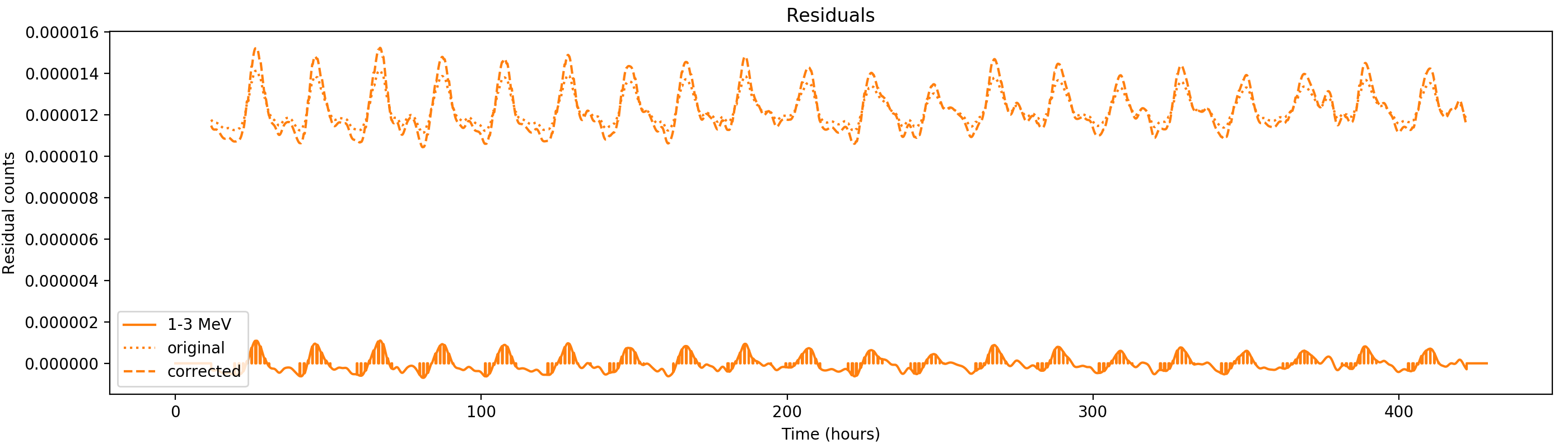
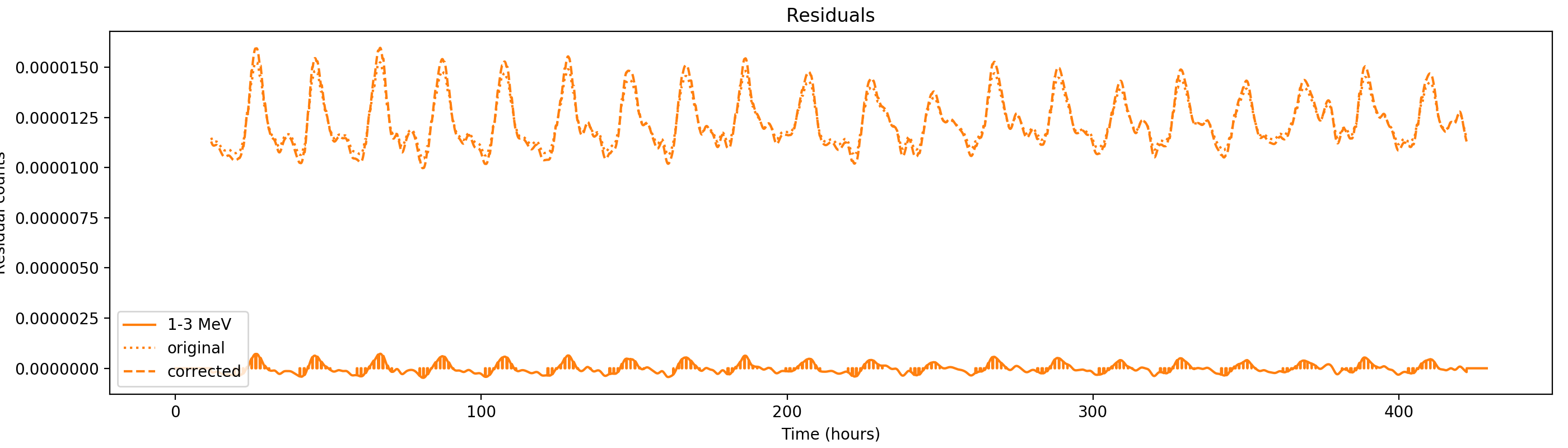
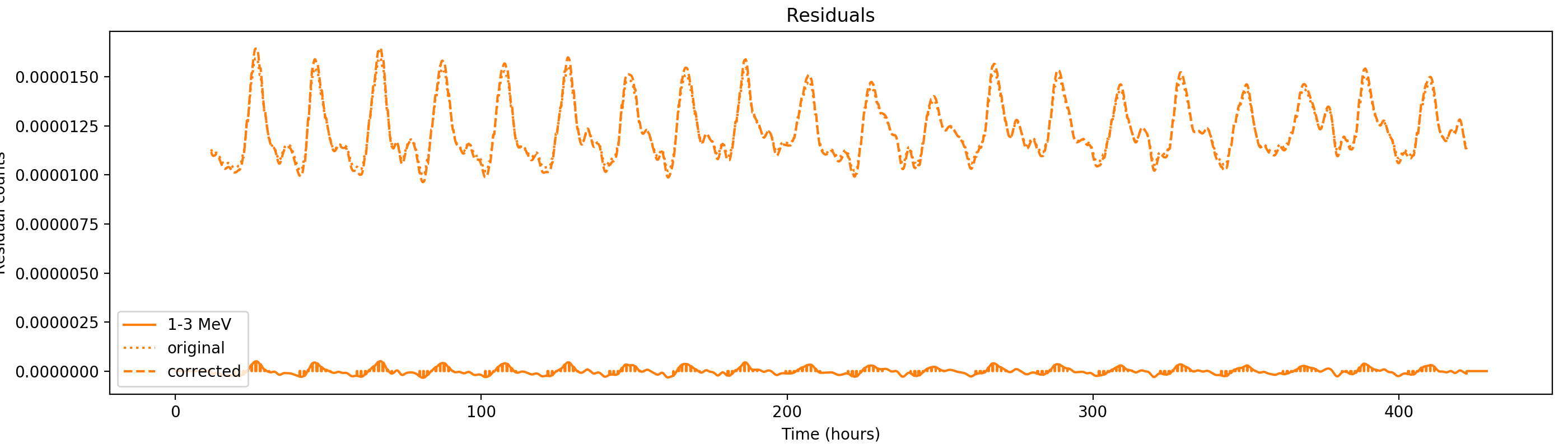
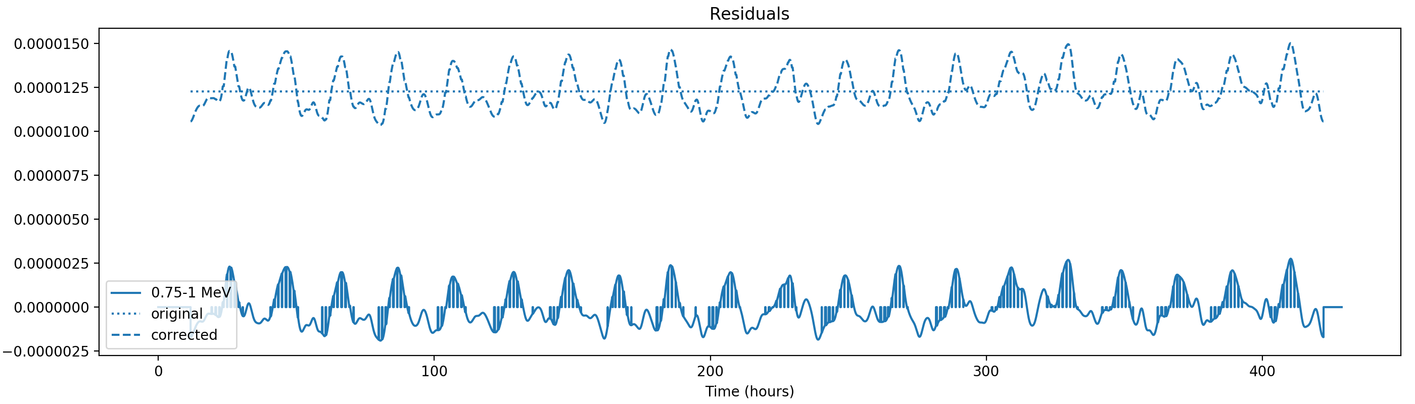
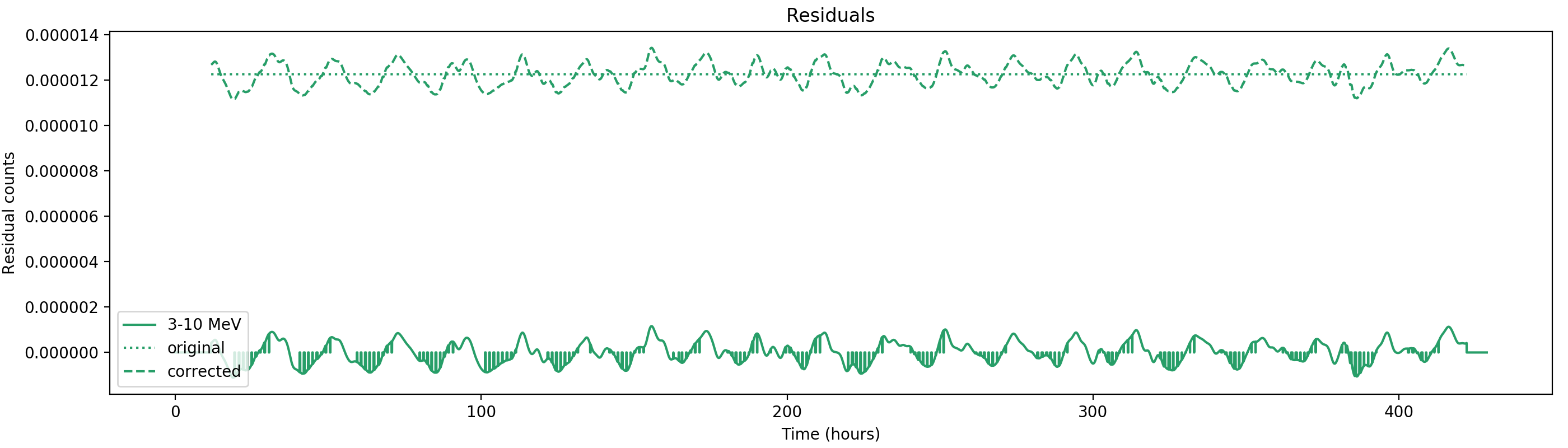
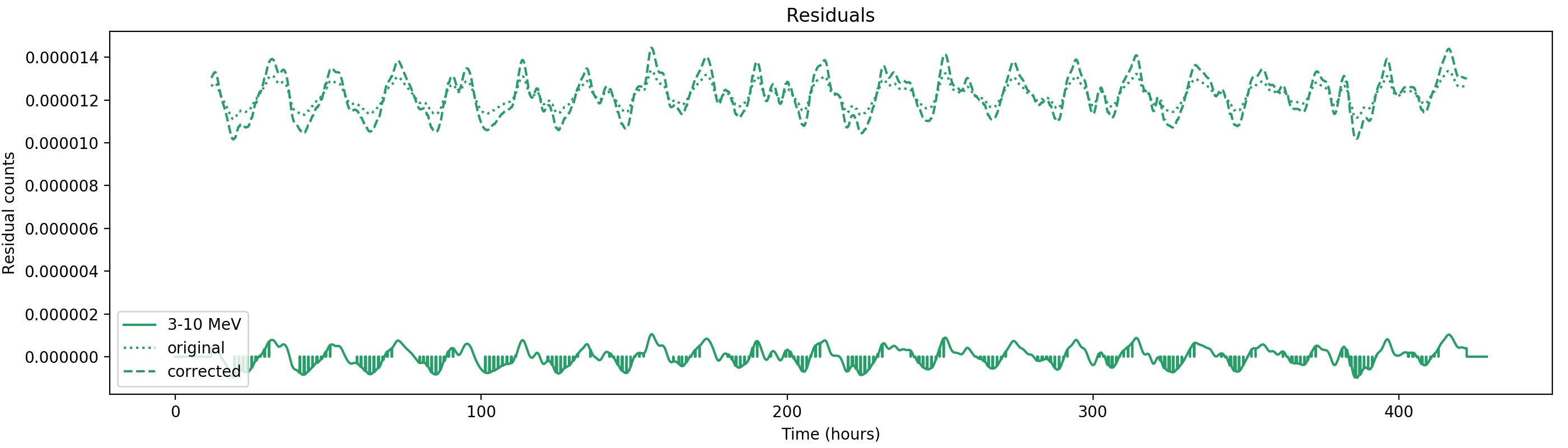
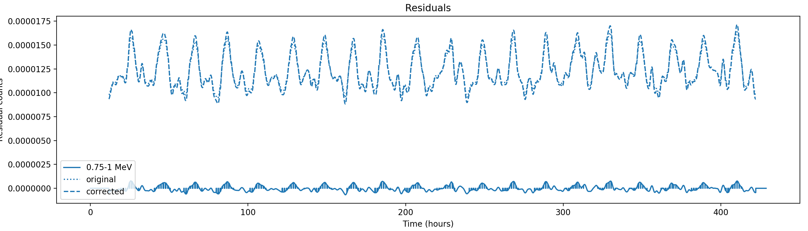
Nevertheless, results are shown below for illustration. The solid line is the residual, with missing data now being visible by vertical lines. The orignal constrate model is shown by a dotted line, the updated model by adding the backprojected residual to the constrate model is shown as dashed line (label using “corrected”). The procedure is repeated 5 times, leading with each iteration to a smaller residual and an improved maximum log-likelihood. The table below shows the evolution of the log-likelihood values and f_prompt.
| 0.75-1 MeV | 1-3 MeV | 3-10 MeV | 10-30 MeV |
 |
 |
 |
 |
 |
 |
 |
 |
 |
 |
 |
 |
 |
 |
 |
 |
 |
 |
 |
 |
| 0.75-1 MeV | 1-3 MeV | 3-10 MeV | 10-30 MeV |
| 206443.354 (0.3895 ± 0.0059) | 852066.391 (0.4876 ± 0.0022) | 525169.470 (0.9090 ± 0.0033) | 136617.278 (1.0000 ± 0.0082) |
| 206140.899 (0.3913 ± 0.0041) | 851207.702 (0.4941 ± 0.0020) | 525124.172 (0.8921 ± 0.0060) | 136617.257 (0.9937 ± 0.0080) |
| 206060.135 (0.4110 ± 0.0039) | 850918.500 (0.5091 ± 0.0019) | 525082.303 (0.8799 ± 0.0057) | 136610.807 (0.9459 ± 0.0150) |
| 206026.781 (0.4277 ± 0.0040) | 850794.903 (0.5210 ± 0.0019) | 525047.029 (0.8724 ± 0.0055) | 136597.583 (0.9121 ± 0.0133) |
| 206008.808 (0.4392 ± 0.0041) | 850733.557 (0.5308 ± 0.0019) | 525018.735 (0.8683 ± 0.0053) | 136583.161 (0.8922 ± 0.0120) |
#23
Updated by Knödlseder Jürgen almost 2 years ago
- File corrected3-fc1-gauss1h-1st.png added
- File corrected3-fc1-gauss1h-2nd.png added
- File corrected3-fc1-gauss1h-3rd.png added
- File corrected3-fc1-gauss1h-4th.png added
- File corrected3-fc1-gauss1h-5th.png added
- File corrected2-fc1-gauss1h-4th.png added
- File corrected2-fc1-gauss1h-5th.png added
- File corrected0-fc1-gauss1h-3rd.png added
- File corrected0-fc1-gauss1h-4th.png added
- File corrected0-fc1-gauss1h-5th.png added
#24
Updated by Knödlseder Jürgen almost 2 years ago
Following the implementation of the code in GCOMDris, here the result. It is again disappointing that the residuals were only very marginally improved. I still need to check that the code does what it is expected to do, but I had hoped for a more important impact.
| Configuration | 0.75-1 MeV | 1-3 MeV | 3-10 MeV | 10-30 MeV |
| BGDLIXE | -5.23 - 5.02 | -6.94 - 7.58 | -4.22 - 4.03 | -3.35 - 3.44 |
| BGDLIXF, EHACORR<10, 300 sec | -4.75 - 4.35 | -5.14 - 5.91 | -3.55 - 3.67 | -3.38 - 3.46 |
| BGDLIXF, VETORATE (initial) | -4.89 - 4.65 | -5.22 - 6.40 | -3.43 - 3.67 | -3.20 - 3.34 |
| BGDLIXF, VETORATE (activ, 5 iter, 1h) | -4.85 - 4.60 | -5.15 - 6.31 | -3.41 - 3.65 | -3.22 - 3.34 |

#25
Updated by Knödlseder Jürgen almost 2 years ago
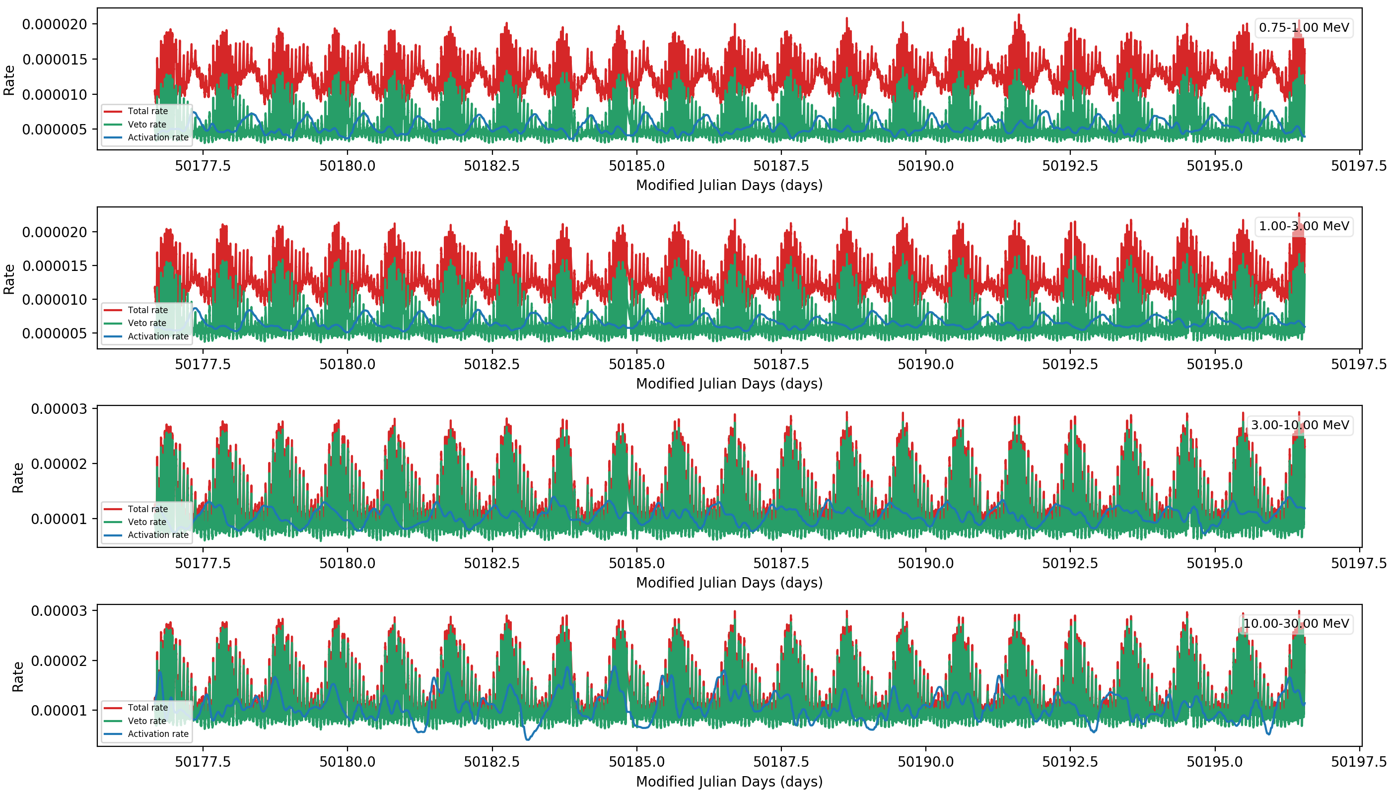
- File drw-rates.png added
- % Done changed from 60 to 70
Here the rates in the DRW files, the computation seems correct and corresponds to the results shown above that were derived using a Python script. Interestingly, for the two lower energy bands the activation follows the peaks in the veto rates, which is reasonable since the activation happens due to prompt background that is higher close to the SAA. For the two upper bands, the activation aligns with the Veto rate peaks, illustrating that the iterative residual rate corrections primarily compensate for residuals during the Veto rate peaks, and do not correspond to actual activation. The smallness of the activation corrections may explain why there is in fact no significant improvement of the background residuals with this improved handling: the related rate variations are in fact not very large, making this rather a second order effect.

#26
Updated by Knödlseder Jürgen almost 2 years ago
I repeated the analysis for Gaussian smoothing kernels with sigma = 30 min and 2 hours. The length of the smoothing kernel has little impact on the results, as expected for the case that the activation correction has little impact on the residuals.
| Configuration | 0.75-1 MeV | 1-3 MeV | 3-10 MeV | 10-30 MeV |
| BGDLIXE | -5.23 - 5.02 | -6.94 - 7.58 | -4.22 - 4.03 | -3.35 - 3.44 |
| BGDLIXF, EHACORR<10, 300 sec | -4.75 - 4.35 | -5.14 - 5.91 | -3.55 - 3.67 | -3.38 - 3.46 |
| BGDLIXF, VETORATE (initial) | -4.89 - 4.65 | -5.22 - 6.40 | -3.43 - 3.67 | -3.20 - 3.34 |
| BGDLIXF, VETORATE (activ, 5 iter, 1h) | -4.85 - 4.60 | -5.15 - 6.31 | -3.41 - 3.65 | -3.22 - 3.34 |
| BGDLIXF, VETORATE (activ, 5 iter, 30min) | -4.86 - 4.60 | -5.15 - 6.31 | -3.40 - 3.65 | -3.23 - 3.35 |
| BGDLIXF, VETORATE (activ, 5 iter, 2h) | -4.85 - 4.60 | -5.16 - 6.33 | -3.42 - 3.65 | -3.21 - 3.34 |
- taking into account the time variation of the event rate in the background modelling reduces somewhat the background residuals
- deriving an energy-independent time variation at a scale of 5 minutes (
phibarmethod) leads to results that are equivalent to a model based on the veto rate and a correction for activation in the SAA (vetoratemethod) - some background residuals persist, suggesting that they come from an inadequacy of the model that does not relate to the time-variation of the event rate; since the residuals are only occurring for the two lower energy bands it is plausible that the residuals come from activation, and may have to do with difference of the event rate distribution with respect to the geometry function
In conclusion, it seems not possible to improve the current background model any further without reconsidering the hypothesis that the event rate follows the geometry function.