Action #742

Feature #735: Implement SPI response interface
Implement GSPIResponse
| Status: | Closed | Start date: | ||
|---|---|---|---|---|
| Priority: | Normal | Due date: | ||
| Assigned To: |  Knödlseder Jürgen Knödlseder Jürgen | % Done: | 100% | |
| Category: | - | |||
| Target version: | 1.7.0 | |||
| Duration: |
GSPIResponse_irf_check1.png (98.1 KB)
GSPIResponse_irf_check2.png (238 KB)
test_irf_method.py  (2.07 KB)
test_crab_fit.py
(1.42 KB)
map_elliptical_iter4-4.png (71.2 KB)
map_elliptical_iter6-6.png (72.3 KB)
map_elliptical_iter5-5.png (68.3 KB)
map_elliptical_iter7-7.png (73 KB)


Recurrence
No recurrence.
History
#1
 Updated by Knödlseder Jürgen about 11 years ago
- Target version deleted (
SPI sprint #1)
#2
Updated by Knödlseder Jürgen almost 5 years ago
- Assigned To set to Knödlseder Jürgen
- Target version set to 1.7.0
#3
Updated by Knödlseder Jürgen almost 5 years ago
- Status changed from New to In Progress
spi_toolslib, hence it should be possible to extract it from there. Here some relevant methods:
SPIResponse::getPointSource: get response for a point source at a positionxandyin Galactic coordinates (deg) and for an energy bin[pmin, pmax]SPIResponse::get_response: get response for a given pointing, zenith and azimuth angle and energy boundarySPIResponse::add_response: add response for a given pointing (computesData_i = Data_i + Response_ij)SPIResponse::get_irf: get IRF for all pseudo-detectors and energy binsSPIResponse::get_irf_pre_calc: get IRF for pre-calculated responseSPIResponse::get_irf_on_the_fly: get IRF from on-the-fly computationSPIResponse::get_irf_value: bilinear interpolation of IRF value in precalculated IRF arraySPIResponse::irf: floating point array with IRFs calculated for all energy binsSPIResponse::init_irf: sets up the response from the response group file for all energy bins in the observation. This is the master method that converts the SPI response data into theirfarrays that are used internally. That’s the point where we have to start.
#4
Updated by Knödlseder Jürgen almost 5 years ago
We need to satisfy the call to the method
double GSPIResponse::irf(const GEvent& event, const GPhoton& photon, const GObservation& obs) const
GPhoton comprised of a sky direction GSkyDir, an energy GEnergy and a time GTime.
For a sky model, the computation of the model values goes via the GModelSky::eval() method that calls the GResponse::convolve() method. Without energy dispersion the later method assigns the measured energy as the true energy
// Get source energy (no dispersion)
GEnergy srcEng  = event.energy();
spi_toolslib assuming that the “imaging space” energy binning is the same as the “data space” energy binning. In that case, the precomputed response is a 4d array, with two spatial dimensions (the original SPI IRFs have 95 x 95 pixels), one detector dimension (85 at most, but typically only 19 for SE) and one energy dimension (the number of energy bins in the “data space”).
The only issue is then whether an energy band or a line response should be used. A flag can certainly be added to toggle between these possibilities. Also, it should be possible to specify a line energy. Alternatively, a line energy could be used automatically if only a single energy bin is present. But this would leave less control to the user...
In case that energy dispersion should be used, pre computation is not effective. Then only the relevant IRFs should be loaded (the ones that correspond to the detectors that are available in the “data space”).
#5
Updated by Knödlseder Jürgen almost 5 years ago
- % Done changed from 0 to 10
Note that the IRF FITS files mention that the x and y axis are given in zenith equidistance. This should correspond to the WCS ARC projection.
The method SPIResponse::get_irf() which takes the zenith and azimuth angle as arguments compute the position in the x and y axis as follows:
// Get position in IRF array in units of IRF pixels.
double xpos = (zenith * cos(azimuth) - irf_xmin) / irf_xbin;
double ypos = (zenith * sin(azimuth) - irf_ymin) / irf_ybin;
Here the relevant coordinate transformation code in spi_toolslib:
typedef struct {                 // SPI coordinate transformation
    double ra_x;                   // X-axis R.A. or Longitude (radians)
    double dec_x;                  // X-axis Dec. or Latitude (radians)
    double ra_y;                   // Y-axis R.A. or Longitude (radians)
    double dec_y;                  // Y-axis Dec. or Latitude (radians)
    double ra_z;                   // Z-axis R.A. or Longitude (radians)
    double dec_z;                  // Z-axis Dec. or Latitude (radians)
    double sin_dec_x;              // sin(dec_x)
    double cos_dec_x;              // cos(dec_x)
    double sin_dec_y;              // sin(dec_y)
    double cos_dec_y;              // cos(dec_y)
    double sin_dec_z;              // sin(dec_z)
    double cos_dec_z;              // cos(dec_z)
    double cos_x_a;                // sin(dec_x) * sin(dec)
    double cos_x_b;                // cos(dec_x) * cos(dec)
    double cos_y_a;                // sin(dec_y) * sin(dec)
    double cos_y_b;                // cos(dec_y) * cos(dec)
    double cos_z_a;                // sin(dec_z) * sin(dec)
    double cos_z_b;                // cos(dec_z) * cos(dec)
} SPICotra;
void cotra_set_pointing(double ra_x, double dec_x, double ra_z, double dec_z, const SPICoordSys& cosys, SPICotra* cotra)
{
    // If requested, transform SPI X- and Z-axes in galactic coordinate
    // system
    if (cosys == SPI_GALACTIC) {
      slaEqgal(ra_x, dec_x, &(cotra->ra_x), &(cotra->dec_x));
      slaEqgal(ra_z, dec_z, &(cotra->ra_z), &(cotra->dec_z));
    }

    // ... otherwise just store coordinates
    else {
      cotra->ra_x  = ra_x;
      cotra->dec_x = dec_x;
      cotra->ra_z  = ra_z;
      cotra->dec_z = dec_z;
    }

    // Calculate SPI Y-axis (radians)
    double xvec[3];
    double yvec[3];
    double zvec[3];
    slaDcs2c(cotra->ra_x, cotra->dec_x, xvec);
    slaDcs2c(cotra->ra_z, cotra->dec_z, zvec);
    slaDvxv(zvec, xvec, yvec);
    slaDcc2s(yvec, &(cotra->ra_y), &(cotra->dec_y));
    cotra->ra_y = slaDranrm(cotra->ra_y);

    // Calculate sine and cosine of X,Y,Z-axes declinations
    cotra->sin_dec_x = sin(cotra->dec_x);
    cotra->cos_dec_x = cos(cotra->dec_x);
    cotra->sin_dec_y = sin(cotra->dec_y);
    cotra->cos_dec_y = cos(cotra->dec_y);
    cotra->sin_dec_z = sin(cotra->dec_z);
    cotra->cos_dec_z = cos(cotra->dec_z);

    // Return
    return;

}
void cotra_set_declination(const double& sin_dec, const double& cos_dec, SPICotra* cotra)
{
    // Precompute declination factors for coordinate transformation
    cotra->cos_x_a = cotra->sin_dec_x * sin_dec;
    cotra->cos_x_b = cotra->cos_dec_x * cos_dec;
    cotra->cos_y_a = cotra->sin_dec_y * sin_dec;
    cotra->cos_y_b = cotra->cos_dec_y * cos_dec;
    cotra->cos_z_a = cotra->sin_dec_z * sin_dec;
    cotra->cos_z_b = cotra->cos_dec_z * cos_dec;

    // Return
    return;

}
void cotra_get_spherical(const double& ra, SPICotra* cotra, double* zenith, double* azimuth)
{
    // Compute zenith and azimuth angles of pixel in instrument system
    double cos_ra_x = cos(cotra->ra_x - ra);
    double cos_x    = cotra->cos_x_a + cotra->cos_x_b * cos_ra_x;
    double cos_ra_y = cos(cotra->ra_y - ra);
    double cos_y    = cotra->cos_y_a + cotra->cos_y_b * cos_ra_y;
    double cos_ra_z = cos(cotra->ra_z - ra);
    double cos_z    = cotra->cos_z_a + cotra->cos_z_b * cos_ra_z;
    if (cos_x >  1.0) cos_x =  1.0;
    if (cos_x < -1.0) cos_x = -1.0;
    if (cos_y >  1.0) cos_y =  1.0;
    if (cos_y < -1.0) cos_y = -1.0;
    if (cos_z >  1.0) cos_z =  1.0;
    if (cos_z < -1.0) cos_z = -1.0;
    *zenith  = acos(cos_x);
    *azimuth = atan2(cos_z, cos_y);
    if (*azimuth < 0.0) *azimuth += twopi;

    // Return
    return;

}
which is used as follows in
SPIResponse::getPointSource: // Determine source Right Ascension and Declination in radians
x *= deg2rad;
y *= deg2rad;
if (system == SPI_GALACTIC) {
double x_out;
double y_out;
slaGaleq(x, y, &x_out, &y_out);
x = x_out;
y = y_out;
}
double sin_y = sin(y);
double cos_y = cos(y);
// Loop over all pointings
for (int ipt = 0; ipt < dat_pt_num; ++ipt) {
// Initialise coordinate transformation
SPICotra cotra;
cotra_set_pointing(aux_ra_spix[ipt], aux_dec_spix[ipt], aux_ra_spiz[ipt], aux_dec_spiz[ipt], SPI_CELESTIAL, &cotra);
// Get bounding box for actual pointing in image coordinate system
SPIBoundingBox box;
cotra_get_bounding_box(&cotra, par_max_zenith, &box);
// Skip if we're outside the relevant range
if (not_in_y_boundary(&box, y) || not_in_x_boundary(&box, x))
continue;
// Precompute declination factors for coordinate transformation
cotra_set_declination(sin_y, cos_y, &cotra);
// Compute zenith and azimuth angles of pixel in instrument system
double zenith;
double azimuth;
cotra_get_spherical(x, &cotra, &zenith, &azimuth);
// Skip pixel if zenith angle exceeds the maximum zenith angle
if (zenith > par_max_zenith)
continue;
// Get response for all detetors and energy bins
get_response(ipt, zenith, azimuth, pmin, pmax, det_counts);
// Add response
add_response(ipt, det_counts, data);
} // endfor: Looped over all telescope pointings
#6
Updated by Knödlseder Jürgen almost 5 years ago
- % Done changed from 10 to 30
I implemented the IRF loading and pre-computation in GSPIResponse. The implemented code corresponds to the SPIResponse::init_irf() method of spi_toolslib.
#7
Updated by Knödlseder Jürgen almost 5 years ago
- File GSPIResponse_irf_check1.png added
- File GSPIResponse_irf_check2.png added
- File test_irf_method.py added
- % Done changed from 30 to 50
I implemented the IRF computation in GSPIResponse. Specifically, the method
double GSPIResponse::irf(const GSkyDir& srcDir, const GSPIEventBin& bin, const int& ireg) const
ireg parameter.
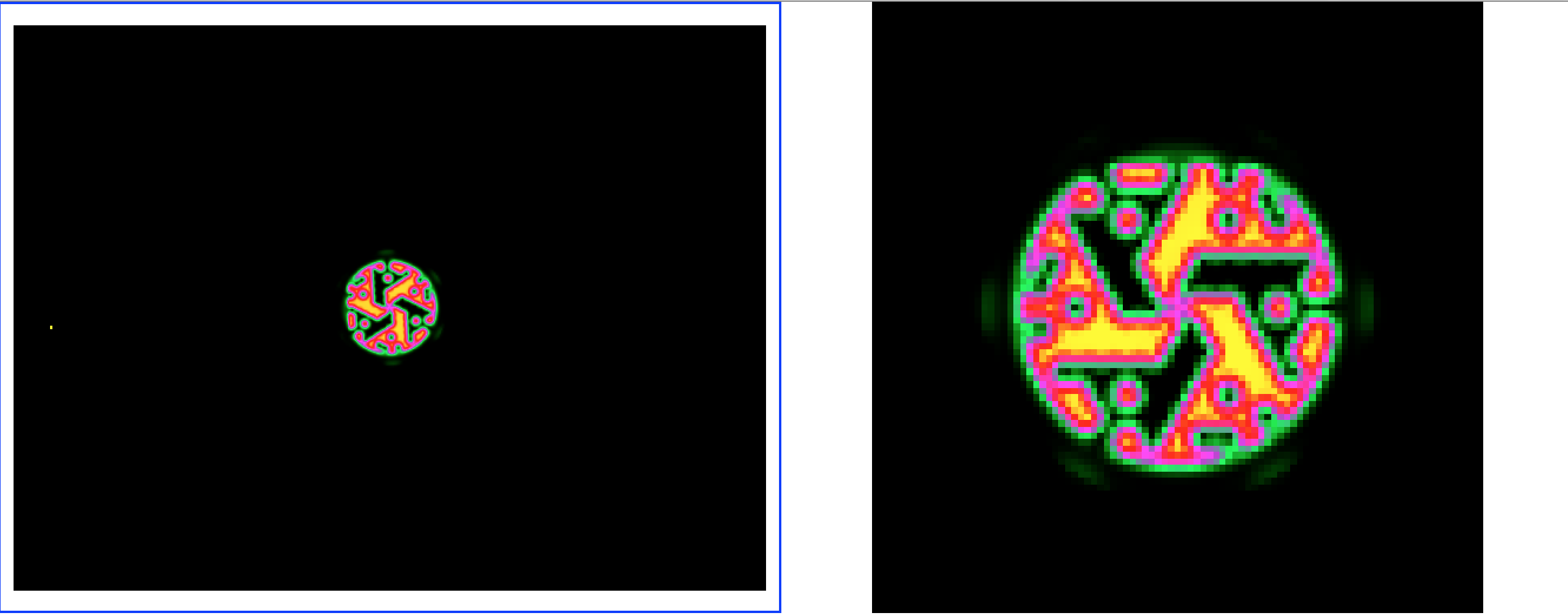
I checked the method using the script test_irf_method.py. The script produces a sky map for the first event found in an observation. The sky map is centred on the SPI pointing direction for that event. Thus, the map should show the IRF centred on the map centre and rotated by an angle that corresponds to the orientation of the telescope. To check the orientation I also plotted the SPI Z axis as yellow square on the map.
The figure below shows the result of this check. The left panel shows the sky map generated using the script, the right panel shows the IRF from the response files. The telescope Z axis in the response files is facing up. It is obvious that when the left panel is rotated clockwise so that the yellow square faces up, both IRF images do match. The image in the left panel is much smoother since the response was computed on a grid of 0.1 deg, and the GSPIResponse::irf() method performs a bilinear interpolation of the response, similar to what is done in spi_toolslib.

To check that the IRF is also well aligned I plotted also the SPI X axis as yellow cross on the map. Zooming-in produces the figure below. The width of the cross is 0.1 deg, the original pixel size of the IRF is 0.5 deg. Would there be an offset by one pixel in the response computation, the centre of the mask would be displaced by five times the thickness of the cross. This is obviously not the case, hence the IRF seems to be correctly aligned.

#8
Updated by Knödlseder Jürgen almost 5 years ago
- File test_crab_fit.py added
- % Done changed from 50 to 60
And here is the first ctlike result on the SPI test data set. The Crab was fit as a point source with a power-law spectral model. The position of the point source was left free. The fitted position is offset by about 1 arcmin from the true position, as illustrated in the table below that summarises the results. This reaffirms that the spatial alignment of the IRF computation is accurate.
| Parameter | ctlike | Simbad | ctlike offset |
| Right Ascension | 83.64274 +/- 0.00843 | 83.63308 | +0.00966 |
| Declination | 22.03462 +/- 0.00769 | 22.01450 | +0.02012 |
2020-04-09T13:19:09: +===================+
2020-04-09T13:19:09: | Input observation |
2020-04-09T13:19:09: +===================+
2020-04-09T13:19:09: === GObservations ===
2020-04-09T13:19:09:  Number of observations ....: 1
2020-04-09T13:19:09:  Number of models ..........: 2
2020-04-09T13:19:09:  Number of observed events .: 101269457
2020-04-09T13:19:09:  Number of predicted events : 0
2020-04-09T13:19:09: === GSPIObservation ===
2020-04-09T13:19:09:  Name ......................:
2020-04-09T13:19:09:  Identifier ................:
2020-04-09T13:19:09:  Instrument ................: SPI
2020-04-09T13:19:09:  Statistic .................: cstat
2020-04-09T13:19:09:  Ontime ....................: 193966.817867279 sec
2020-04-09T13:19:09:  Livetime ..................: 170657.53716056 sec
2020-04-09T13:19:09:  Deadtime correction .......: 0.879828514160249
2020-04-09T13:19:09: === GSPIEventCube ===
2020-04-09T13:19:09:  Number of events ..........: 101269457
2020-04-09T13:19:09:  Number of elements ........: 16720
2020-04-09T13:19:09:  Pointings .................: 88
2020-04-09T13:19:09:  Detectors .................: 19
2020-04-09T13:19:09:  Energy bins ...............: 10
2020-04-09T13:19:09:  Sky models ................: 0
2020-04-09T13:19:09:  Background models .........: 1
2020-04-09T13:19:09:   Model name 1 .............: String
2020-04-09T13:19:09:   Number of events .........: 101269456.964783
2020-04-09T13:19:09:  Energy range ..............: 0.05 - 1 MeV
2020-04-09T13:19:09:  Ontime ....................: 193966.817867279 s
2020-04-09T13:19:09:  Livetime ..................: 170657.53716056 s
2020-04-09T13:19:09:  Time interval .............: 2003-02-22T04:06:19 - 2003-02-24T16:17:19
2020-04-09T13:19:09:
2020-04-09T13:19:09: +=================================+
2020-04-09T13:19:09: | Maximum likelihood optimisation |
2020-04-09T13:19:09: +=================================+
2020-04-09T13:19:09:  >Iteration   0: -logL=-795434690.331, Lambda=1.0e-03
2020-04-09T13:19:09:   Iteration   1: -logL=-795434690.331, Lambda=1.0e-03, delta=-158968958130.947, step=1.0e+00, max(|grad|)=-669321217639.636963 [Index:3] (stalled)
2020-04-09T13:19:09:   Iteration   2: -logL=-795434690.331, Lambda=1.0e-02, delta=-55025202657.712, step=1.0e+00, max(|grad|)=-230748454256.151367 [Index:3] (stalled)
2020-04-09T13:19:09:   Iteration   3: -logL=-795434690.331, Lambda=1.0e-01, delta=-15887675.016, step=1.0e+00, max(|grad|)=-89025790.206532 [Index:3] (stalled)
2020-04-09T13:19:09:   Iteration   4: -logL=-795434690.331, Lambda=1.0e+00, delta=-5781.546, step=1.0e+00, max(|grad|)=36435.007074 [GEDSAT D018 Rev0044:24] (stalled)
2020-04-09T13:19:09:  >Iteration   5: -logL=-795437088.825, Lambda=1.0e+01, delta=2398.494, step=1.0e+00, max(|grad|)=8879.053950 [GEDSAT D003 Rev0044:9]
2020-04-09T13:19:09:   Iteration   6: -logL=-795437088.825, Lambda=1.0e+00, delta=-9195.831, step=1.0e+00, max(|grad|)=23875.550066 [GEDSAT D010 Rev0044:16] (stalled)
2020-04-09T13:19:09:  >Iteration   7: -logL=-795439273.845, Lambda=1.0e+01, delta=2185.020, step=1.0e+00, max(|grad|)=12370.649685 [GEDSAT D003 Rev0044:9]
2020-04-09T13:19:09:  >Iteration   8: -logL=-795442570.226, Lambda=1.0e+00, delta=3296.381, step=1.0e+00, max(|grad|)=20594.148751 [GEDSAT D018 Rev0044:24]
2020-04-09T13:19:09:   Iteration   9: -logL=-795442570.226, Lambda=1.0e-01, delta=-1214.850, step=1.0e+00, max(|grad|)=-8478.979400 [DEC:1] (stalled)
2020-04-09T13:19:09:  >Iteration  10: -logL=-795446031.387, Lambda=1.0e+00, delta=3461.161, step=1.0e+00, max(|grad|)=11547.775550 [GEDSAT D014 Rev0044:20]
2020-04-09T13:19:09:  >Iteration  11: -logL=-795447639.840, Lambda=1.0e-01, delta=1608.453, step=1.0e+00, max(|grad|)=6841.467639 [DEC:1]
2020-04-09T13:19:09:   Iteration  12: -logL=-795447639.840, Lambda=1.0e-02, delta=-1798.396, step=1.0e+00, max(|grad|)=17047.346849 [GEDSAT D014 Rev0044:20] (stalled)
2020-04-09T13:19:09:   Iteration  13: -logL=-795447639.840, Lambda=1.0e-01, delta=-125.659, step=1.0e+00, max(|grad|)=11310.033497 [GEDSAT D014 Rev0044:20] (stalled)
2020-04-09T13:19:10:  >Iteration  14: -logL=-795451315.872, Lambda=1.0e+00, delta=3676.032, step=1.0e+00, max(|grad|)=5892.392308 [GEDSAT D014 Rev0044:20]
2020-04-09T13:19:10:  >Iteration  15: -logL=-795453506.474, Lambda=1.0e-01, delta=2190.601, step=1.0e+00, max(|grad|)=9040.580297 [GEDSAT D018 Rev0044:24]
2020-04-09T13:19:10:  >Iteration  16: -logL=-795454274.956, Lambda=1.0e-02, delta=768.482, step=1.0e+00, max(|grad|)=-5671.314118 [DEC:1]
2020-04-09T13:19:10:  >Iteration  17: -logL=-795454508.847, Lambda=1.0e-03, delta=233.891, step=1.0e+00, max(|grad|)=5446.377721 [DEC:1]
2020-04-09T13:19:10:  >Iteration  18: -logL=-795454807.932, Lambda=1.0e-04, delta=299.085, step=1.0e+00, max(|grad|)=-4252.947991 [DEC:1]
2020-04-09T13:19:10:   Iteration  19: -logL=-795454807.932, Lambda=1.0e-05, delta=-97.416, step=1.0e+00, max(|grad|)=4378.403658 [DEC:1] (stalled)
2020-04-09T13:19:10:   Iteration  20: -logL=-795454807.932, Lambda=1.0e-04, delta=-97.300, step=1.0e+00, max(|grad|)=4377.965242 [DEC:1] (stalled)
2020-04-09T13:19:10:   Iteration  21: -logL=-795454807.932, Lambda=1.0e-03, delta=-96.143, step=1.0e+00, max(|grad|)=4373.585699 [DEC:1] (stalled)
2020-04-09T13:19:10:   Iteration  22: -logL=-795454807.932, Lambda=1.0e-02, delta=-84.756, step=1.0e+00, max(|grad|)=4330.248361 [DEC:1] (stalled)
2020-04-09T13:19:10:  >Iteration  23: -logL=-795454818.260, Lambda=1.0e-01, delta=10.328, step=1.0e+00, max(|grad|)=3542.607758 [DEC:1]
2020-04-09T13:19:10:  >Iteration  24: -logL=-795454966.453, Lambda=1.0e-02, delta=148.193, step=1.0e+00, max(|grad|)=-3252.606596 [DEC:1]
2020-04-09T13:19:10:   Iteration  25: -logL=-795454966.453, Lambda=1.0e-03, delta=-147.014, step=1.0e+00, max(|grad|)=3418.758519 [DEC:1] (stalled)
2020-04-09T13:19:10:   Iteration  26: -logL=-795454966.453, Lambda=1.0e-02, delta=-140.069, step=1.0e+00, max(|grad|)=3386.639885 [DEC:1] (stalled)
2020-04-09T13:19:10:   Iteration  27: -logL=-795454966.453, Lambda=1.0e-01, delta=-80.187, step=1.0e+00, max(|grad|)=3098.495241 [DEC:1] (stalled)
2020-04-09T13:19:10:  >Iteration  28: -logL=-795455088.189, Lambda=1.0e+00, delta=121.737, step=1.0e+00, max(|grad|)=1419.523198 [DEC:1]
2020-04-09T13:19:10:   Iteration  29: -logL=-795455088.189, Lambda=1.0e-01, delta=-32.806, step=1.0e+00, max(|grad|)=-2467.573153 [DEC:1] (stalled)
2020-04-09T13:19:10:  >Iteration  30: -logL=-795455125.934, Lambda=1.0e+00, delta=37.745, step=1.0e+00, max(|grad|)=-486.971831 [DEC:1]
2020-04-09T13:19:10:   Iteration  31: -logL=-795455125.934, Lambda=1.0e-01, delta=-15.448, step=1.0e+00, max(|grad|)=1049.595829 [DEC:1] (stalled)
2020-04-09T13:19:10:   Iteration  32: -logL=-795455125.934, Lambda=1.0e+00, delta=-4.473, step=1.0e+00, max(|grad|)=849.888147 [DEC:1] (stalled)
2020-04-09T13:19:10:  >Iteration  33: -logL=-795455126.454, Lambda=1.0e+01, delta=0.519, step=1.0e+00, max(|grad|)=193.797739 [DEC:1]
2020-04-09T13:19:11:   Iteration  34: -logL=-795455124.989, Lambda=1.0e+00, delta=-1.464, step=1.0e+00, max(|grad|)=-661.816001 [DEC:1] (stalled)
2020-04-09T13:19:11:  >Iteration  35: -logL=-795455126.894, Lambda=1.0e+01, delta=1.905, step=1.0e+00, max(|grad|)=-483.927449 [DEC:1]
2020-04-09T13:19:11:   Iteration  36: -logL=-795455126.894, Lambda=1.0e+00, delta=-5.870, step=1.0e+00, max(|grad|)=860.647171 [DEC:1] (stalled)
2020-04-09T13:19:11:   Iteration  37: -logL=-795455126.691, Lambda=1.0e+01, delta=-0.203, step=1.0e+00, max(|grad|)=197.947325 [DEC:1] (stalled)
2020-04-09T13:19:11:  >Iteration  38: -logL=-795455126.715, Lambda=1.0e+02, delta=0.024, step=1.0e+00, max(|grad|)=195.924094 [DEC:1]
2020-04-09T13:19:11:  >Iteration  39: -logL=-795455126.924, Lambda=1.0e+01, delta=0.209, step=1.0e+00, max(|grad|)=177.610555 [DEC:1]
2020-04-09T13:19:11:   Iteration  40: -logL=-795455125.146, Lambda=1.0e+00, delta=-1.779, step=1.0e+00, max(|grad|)=-640.327436 [DEC:1] (stalled)
2020-04-09T13:19:11:  >Iteration  41: -logL=-795455126.965, Lambda=1.0e+01, delta=1.819, step=1.0e+00, max(|grad|)=-488.282482 [DEC:1]
2020-04-09T13:19:11:   Iteration  42: -logL=-795455126.965, Lambda=1.0e+00, delta=-5.836, step=1.0e+00, max(|grad|)=858.470501 [DEC:1] (stalled)
2020-04-09T13:19:11:   Iteration  43: -logL=-795455126.965, Lambda=1.0e+01, delta=-0.136, step=1.0e+00, max(|grad|)=194.043498 [DEC:1] (stalled)
2020-04-09T13:19:11:  >Iteration  44: -logL=-795455127.101, Lambda=1.0e+02, delta=0.136, step=1.0e+00, max(|grad|)=-399.915292 [DEC:1]
2020-04-09T13:19:11:   Iteration  45: -logL=-795455127.101, Lambda=1.0e+01, delta=-0.238, step=1.0e+00, max(|grad|)=190.937910 [DEC:1] (stalled)
2020-04-09T13:19:11:  >Iteration  46: -logL=-795455127.169, Lambda=1.0e+02, delta=0.068, step=1.0e+00, max(|grad|)=96.749023 [GEDSAT D018 Rev0044:24]
2020-04-09T13:19:11:   Iteration  47: -logL=-795455127.169, Lambda=1.0e+01, delta=-0.056, step=1.0e+00, max(|grad|)=166.320652 [DEC:1] (stalled)
2020-04-09T13:19:11:  >Iteration  48: -logL=-795455127.176, Lambda=1.0e+02, delta=0.007, step=1.0e+00, max(|grad|)=96.857257 [GEDSAT D018 Rev0044:24]
2020-04-09T13:19:11:  >Iteration  49: -logL=-795455127.178, Lambda=1.0e+01, delta=0.001, step=1.0e+00, max(|grad|)=94.170926 [GEDSAT D018 Rev0044:24]
2020-04-09T13:19:11:
2020-04-09T13:19:11:  +==================+
2020-04-09T13:19:11:  | Curvature matrix |
2020-04-09T13:19:11:  +==================+
2020-04-09T13:19:11:  === GMatrixSparse ===
2020-04-09T13:19:11:   Number of rows ............: 25
2020-04-09T13:19:11:   Number of columns .........: 25
2020-04-09T13:19:11:   Number of nonzero elements : 187
2020-04-09T13:19:11:   Number of allocated cells .: 699
2020-04-09T13:19:11:   Memory block size .........: 512
2020-04-09T13:19:11:   Sparse matrix fill ........: 0.2992
2020-04-09T13:19:11:   Pending element ...........: 0
2020-04-09T13:19:11:   Fill stack size ...........: 0 (none)
2020-04-09T13:19:11:   14355.4873220717, -1693.83491508247, 44.6843757415376, -230.219789951165, 0, 0, -8638.65938630058, ... 4790.39347195264, -666.4954473935, -4360.2995239397, 2139.46626317224, 4428.10809054952, 9167.87123694079, 4513.99411486188
2020-04-09T13:19:11:   -1693.83491508247, 17435.0555369516, -158.519731293467, 676.356891345712, 0, 0, 2131.33224757851, ... 946.693942848587, 8179.31574033662, -10599.0837760446, -5324.19572651882, 1630.5831307255, 5062.00182296843, 8206.96521896998
2020-04-09T13:19:11:   44.6843757415376, -158.519731293467, 182.175904742103, -780.228650982818, 0, 0, 4710.90522804617, ... 4402.78682230623, 4414.13668893275, 4748.47226377536, 4335.71189945368, 4494.13816615803, 4276.61307420658, 4756.57685596306
2020-04-09T13:19:11:   -230.219789951165, 676.356891345712, -780.228650982818, 90647.7292147093, 0, 0, -62240.176501595, ... -57357.8628365196, -57087.4264845466, -61721.3348140256, -56551.2343963216, -58876.9875067132, -55674.1292044166, -61459.453206413
2020-04-09T13:19:11:   0, 0, 0, 0, 0, 0, 0, ... 0, 0, 0, 0, 0, 0, 0
2020-04-09T13:19:11:   0, 0, 0, 0, 0, 0, 0, ... 0, 0, 0, 0, 0, 0, 0
2020-04-09T13:19:11:   -8638.65938630058, 2131.33224757851, 4710.90522804617, -62240.176501595, 0, 0, 5302141.13739067, ... 0, 0, 0, 0, 0, 0, 0
2020-04-09T13:19:11:   ... ... ... ... ... ... ... ... ... ... ... ... ... ... ...
2020-04-09T13:19:11:   4790.39347195264, 946.693942848587, 4402.78682230623, -57357.8628365197, 0, 0, 0, ... 5163943.70275155, 0, 0, 0, 0, 0, 0
2020-04-09T13:19:11:   -666.4954473935, 8179.31574033662, 4414.13668893275, -57087.4264845466, 0, 0, 0, ... 0, 5223920.56641392, 0, 0, 0, 0, 0
2020-04-09T13:19:11:   -4360.2995239397, -10599.0837760446, 4748.47226377536, -61721.3348140256, 0, 0, 0, ... 0, 0, 5379124.73356445, 0, 0, 0, 0
2020-04-09T13:19:11:   2139.46626317223, -5324.19572651882, 4335.71189945368, -56551.2343963216, 0, 0, 0, ... 0, 0, 0, 5304116.54855911, 0, 0, 0
2020-04-09T13:19:11:   4428.10809054952, 1630.5831307255, 4494.13816615803, -58876.9875067132, 0, 0, 0, ... 0, 0, 0, 0, 5221871.47862776, 0, 0
2020-04-09T13:19:11:   9167.87123694079, 5062.00182296843, 4276.61307420658, -55674.1292044166, 0, 0, 0, ... 0, 0, 0, 0, 0, 5313489.13673907, 0
2020-04-09T13:19:11:   4513.99411486187, 8206.96521896998, 4756.57685596306, -61459.453206413, 0, 0, 0, ... 0, 0, 0, 0, 0, 0, 5309400.63249363
2020-04-09T13:19:11:
2020-04-09T13:19:11: +====================================+
2020-04-09T13:19:11: | Maximum likelihood re-optimisation |
2020-04-09T13:19:11: +====================================+
2020-04-09T13:19:11:  >Iteration   0: -logL=-795416111.968, Lambda=1.0e-03
2020-04-09T13:19:11:  >Iteration   1: -logL=-795432387.342, Lambda=1.0e-03, delta=16275.374, step=1.0e+00, max(|grad|)=-2084.132823 [GEDSAT D003 Rev0044:3]
2020-04-09T13:19:11:  >Iteration   2: -logL=-795432393.068, Lambda=1.0e-04, delta=5.726, step=1.0e+00, max(|grad|)=-1.014540 [GEDSAT D003 Rev0044:3]
2020-04-09T13:19:11:  >Iteration   3: -logL=-795432393.068, Lambda=1.0e-05, delta=0.000, step=1.0e+00, max(|grad|)=-0.000010 [GEDSAT D003 Rev0044:3]
2020-04-09T13:19:11:
2020-04-09T13:19:11: +============================================+
2020-04-09T13:19:11: | Maximum likelihood re-optimisation results |
2020-04-09T13:19:11: +============================================+
2020-04-09T13:19:11: === GOptimizerLM ===
2020-04-09T13:19:11:  Optimized function value ..: -795432393.068
2020-04-09T13:19:11:  Absolute precision ........: 0.005
2020-04-09T13:19:11:  Acceptable value decrease .: 2
2020-04-09T13:19:11:  Optimization status .......: converged
2020-04-09T13:19:11:  Number of parameters ......: 19
2020-04-09T13:19:11:  Number of free parameters .: 19
2020-04-09T13:19:11:  Number of iterations ......: 3
2020-04-09T13:19:11:  Lambda ....................: 1e-06
2020-04-09T13:19:11:
2020-04-09T13:19:11: +=========================================+
2020-04-09T13:19:11: | Maximum likelihood optimisation results |
2020-04-09T13:19:11: +=========================================+
2020-04-09T13:19:11: === GOptimizerLM ===
2020-04-09T13:19:11:  Optimized function value ..: -795455127.178
2020-04-09T13:19:11:  Absolute precision ........: 0.005
2020-04-09T13:19:11:  Acceptable value decrease .: 2
2020-04-09T13:19:11:  Optimization status .......: converged
2020-04-09T13:19:11:  Number of parameters ......: 25
2020-04-09T13:19:11:  Number of free parameters .: 23
2020-04-09T13:19:11:  Number of iterations ......: 49
2020-04-09T13:19:11:  Lambda ....................: 1
2020-04-09T13:19:11:  Maximum log likelihood ....: 795455127.178
2020-04-09T13:19:11:  Observed events  (Nobs) ...: 101269457.000
2020-04-09T13:19:11:  Predicted events (Npred) ..: 101270576.936 (Nobs - Npred = -1119.93606585264)
2020-04-09T13:19:11: === GModels ===
2020-04-09T13:19:11:  Number of models ..........: 2
2020-04-09T13:19:11:  Number of parameters ......: 25
2020-04-09T13:19:11: === GModelSky ===
2020-04-09T13:19:11:  Name ......................: Crab
2020-04-09T13:19:11:  Instruments ...............: all
2020-04-09T13:19:11:  Test Statistic ............: 45468.2193107605
2020-04-09T13:19:11:  Observation identifiers ...: all
2020-04-09T13:19:11:  Model type ................: PointSource
2020-04-09T13:19:11:  Model components ..........: "PointSource" * "PowerLaw" * "Constant"
2020-04-09T13:19:11:  Number of parameters ......: 6
2020-04-09T13:19:11:  Number of spatial par's ...: 2
2020-04-09T13:19:11:   RA .......................: 83.6427382308396 +/- 0.00842650913652459 deg (free,scale=1)
2020-04-09T13:19:11:   DEC ......................: 22.0346222199456 +/- 0.00769404621003139 deg (free,scale=1)
2020-04-09T13:19:11:  Number of spectral par's ..: 3
2020-04-09T13:19:11:   Prefactor ................: 0.000202043346609174 +/- 9.75244270464002e-07 [0,infty[ ph/cm2/s/MeV (free,scale=1e-05,gradient)
2020-04-09T13:19:11:   Index ....................: -1.49623820737446 +/- 0.0071859668600476 [10,-10]  (free,scale=-2,gradient)
2020-04-09T13:19:11:   PivotEnergy ..............: 0.1 MeV (fixed,scale=0.1,gradient)
2020-04-09T13:19:11:  Number of temporal par's ..: 1
2020-04-09T13:19:11:   Normalization ............: 1 (relative value) (fixed,scale=1,gradient)
2020-04-09T13:19:11:  Number of scale par's .....: 0
2020-04-09T13:19:11: === GSPIModelDataSpace ===
2020-04-09T13:19:11:  Name ......................: GEDSAT
2020-04-09T13:19:11:  Instruments ...............: SPI
2020-04-09T13:19:11:  Observation identifiers ...: all
2020-04-09T13:19:11:  Method ....................: orbit,dete
2020-04-09T13:19:11:  Number of parameters ......: 19
2020-04-09T13:19:11:   GEDSAT D000 Rev0044 ......: 0.981640120395655 +/- 0.00044579620510821  (free,scale=1,gradient)
2020-04-09T13:19:11:   GEDSAT D001 Rev0044 ......: 0.981561830511198 +/- 0.000444137534830371  (free,scale=1,gradient)
2020-04-09T13:19:11:   GEDSAT D002 Rev0044 ......: 0.982056567216066 +/- 0.000441666530430933  (free,scale=1,gradient)
2020-04-09T13:19:11:   GEDSAT D003 Rev0044 ......: 0.980810752069915 +/- 0.000442970422535423  (free,scale=1,gradient)
2020-04-09T13:19:11:   GEDSAT D004 Rev0044 ......: 0.982374553960272 +/- 0.000441071738644522  (free,scale=1,gradient)
2020-04-09T13:19:11:   GEDSAT D005 Rev0044 ......: 0.982304595067843 +/- 0.000441952683082448  (free,scale=1,gradient)
2020-04-09T13:19:11:   GEDSAT D006 Rev0044 ......: 0.983207030065399 +/- 0.000440383922328818  (free,scale=1,gradient)
2020-04-09T13:19:11:   GEDSAT D007 Rev0044 ......: 0.981538989612215 +/- 0.000447214723314897  (free,scale=1,gradient)
2020-04-09T13:19:11:   GEDSAT D008 Rev0044 ......: 0.983381892236331 +/- 0.000440988284838821  (free,scale=1,gradient)
2020-04-09T13:19:11:   GEDSAT D009 Rev0044 ......: 0.982761247901735 +/- 0.000440809414505874  (free,scale=1,gradient)
2020-04-09T13:19:11:   GEDSAT D010 Rev0044 ......: 0.982182387684862 +/- 0.000440759413426911  (free,scale=1,gradient)
2020-04-09T13:19:11:   GEDSAT D011 Rev0044 ......: 0.98104791252 +/- 0.000441632888871981  (free,scale=1,gradient)
2020-04-09T13:19:11:   GEDSAT D012 Rev0044 ......: 0.982302840186701 +/- 0.000450204174219497  (free,scale=1,gradient)
2020-04-09T13:19:11:   GEDSAT D013 Rev0044 ......: 0.982554506946765 +/- 0.000447884449419503  (free,scale=1,gradient)
2020-04-09T13:19:11:   GEDSAT D014 Rev0044 ......: 0.981781432481879 +/- 0.000442211781099953  (free,scale=1,gradient)
2020-04-09T13:19:11:   GEDSAT D015 Rev0044 ......: 0.983031515757366 +/- 0.0004435055783587  (free,scale=1,gradient)
2020-04-09T13:19:11:   GEDSAT D016 Rev0044 ......: 0.982177139235848 +/- 0.00044804494942777  (free,scale=1,gradient)
2020-04-09T13:19:11:   GEDSAT D017 Rev0044 ......: 0.983380843076596 +/- 0.000443342600986916  (free,scale=1,gradient)
2020-04-09T13:19:11:   GEDSAT D018 Rev0044 ......: 0.981538165661823 +/- 0.000445691522464772  (free,scale=1,gradient)
2020-04-09T13:19:11:
2020-04-09T13:19:11: +==============+
2020-04-09T13:19:11: | Save results |
2020-04-09T13:19:11: +==============+
2020-04-09T13:19:11:  Model definition file .....: ctlike.xml
2020-04-09T13:19:11:  Covariance matrix file ....: NONE
2020-04-09T13:19:11:
2020-04-09T13:19:11: Application "ctlike" terminated after 2 wall clock seconds, consuming 2.43981 seconds of CPU time.
The script I used to generate the result is here attachment:test_crab_fit.py.
#9
Updated by Knödlseder Jürgen almost 5 years ago
Obviously, the spectral part is not yet okay. Comparing with Sizun et al. (2004) here is what we expect compared to what we got.
| Parameter | Sizun et al. (2004) | ctlike |
| Prefactor (100 keV) | 0.66 ph/cm2/s/MeV | 2.02043e-4 +/- 0.00975e-4 |
| Index | 2.169 +/- 0.008 | 1.496 +/- 0.007 |
There is obviously a problem with the units. The units of the IRF that are stored in the response files is cm^2. For the moment we multiply the IRFs with the livetime, similar to what is done in spi_toolslib. However, spi_toolslib uses the IRF result directly for model fitting (to be checked), while model values in gammalib are multiplied by the “size” of the event:
model *= bin->size();
#10
Updated by Knödlseder Jürgen almost 5 years ago
I now changed the logic. There is no multiplication with livetime in the IRF anymore, hence they now return simply units of cm^2.
The event bin size is now defined as livetime times energy bin width, hence the model value in GObservation::likelihood_poisson_binned() is now in units of
cm^2 s MeV / ph cm^-2 s-1 MeV-1 = ph
The fit results are now
2020-04-09T14:05:57: === GModelSky ===
2020-04-09T14:05:57:  Name ......................: Crab
2020-04-09T14:05:57:  Instruments ...............: all
2020-04-09T14:05:57:  Test Statistic ............: 45573.9056241512
2020-04-09T14:05:57:  Observation identifiers ...: all
2020-04-09T14:05:57:  Model type ................: PointSource
2020-04-09T14:05:57:  Model components ..........: "PointSource" * "PowerLaw" * "Constant"
2020-04-09T14:05:57:  Number of parameters ......: 6
2020-04-09T14:05:57:  Number of spatial par's ...: 2
2020-04-09T14:05:57:   RA .......................: 83.6474229456721 +/- 0.00822349654274058 deg (free,scale=1)
2020-04-09T14:05:57:   DEC ......................: 22.0306481328862 +/- 0.0077428380097156 deg (free,scale=1)
2020-04-09T14:05:57:  Number of spectral par's ..: 3
2020-04-09T14:05:57:   Prefactor ................: 0.479575170907974 +/- 0.00229067815486417 [0,infty[ ph/cm2/s/MeV (free,scale=1,gradient)
2020-04-09T14:05:57:   Index ....................: -1.45350541199238 +/- 0.00682750950382642 [10,-10]  (free,scale=-2,gradient)
2020-04-09T14:05:57:   PivotEnergy ..............: 0.1 MeV (fixed,scale=0.1,gradient)
2020-04-09T14:05:57:  Number of temporal par's ..: 1
2020-04-09T14:05:57:   Normalization ............: 1 (relative value) (fixed,scale=1,gradient)
2020-04-09T14:05:57:  Number of scale par's .....: 0
The Prefactor result of
0.4796 +/- 0.0023 is now sufficiently close to the value of 0.66 in Sizun et al. (2004). The remaining discrepancy is likely due to the fact that energy dispersion is not yet taken into account, which however is important for SPI.#11
Updated by Knödlseder Jürgen almost 5 years ago
I now did a comparison of a 511 keV line fit between spi_obs_fit and ctlike. A single point source was fitted at the position of the Galactic centre. A 511 keV line response was computed, and for the ctlike model fit a spectral model with a constant was used. Since the ctlike flux is given in units of ph/cm2/s/MeV it needs to be multiplied with the analysis band width of 7 keV to get the line flux.
The results are summarised in table below. They are basically identical, and it’s a good news that also the CPU time consumption between both tools is equivalent.
| Parameter | spi_obs_fit | ctlike |
| logL(H1) | -256643377.628 | -256643377.628 |
| logL(H0) | -256643287.777 | -256643287.777 |
| MLR | 179.70304 | 179.70343 |
| Flux | 2.64452e-04 +/- 1.97371e-05 ph/cm2/s | 0.03778 +/- 0.00282 ph/cm2/s/MeV |
| 511 keV line flux | 2.64452e-04 +/- 1.97371e-05 ph/cm2/s | 2.64455e-04 +/- 1.97373e-05 ph/cm2/s |
| CPU (seconds) | 11 | 10.4 |
#12
Updated by Knödlseder Jürgen almost 5 years ago
For the sake of interest, I also did the ctlike model fit using a Gaussian spectral line model. The model is actually evaluated at the logarithmic bin centre of the 507.5 - 514.5 keV energy bin, which is situated at 510.988 keV. As expected, if the line is placed away from the 511 keV centre, the flux goes up (since the model evaluation is done on the tail of the Gaussian line, hence a higher flux is fitted to compensate for the lower flux in the tail of the model).
| Mean | Sigma | MLR | Flux |
| 509.0 | 2.0 | 179.703 | 3.12263e-04 +/- 2.33054e-05 |
| 510.0 | 2.0 | 179.703 | 2.14615e-04 +/- 1.60176e-05 |
| 510.5 | 2.0 | 179.703 | 1.95409e-04 +/- 1.45842e-05 |
| 511.0 | 2.0 | 179.703 | 1.89397e-04 +/- 1.41355e-05 |
| 511.5 | 2.0 | 179.703 | 1.95409e-04 +/- 1.45842e-05 |
| 512.0 | 2.0 | 179.703 | 2.14615e-04 +/- 1.60176e-05 |
| 513.0 | 2.0 | 179.703 | 3.12263e-04 +/- 2.33054e-05 |
I also compared the 511 keV line response to the continuum response. The results are basically identical.
| Parameter | Line response | Continuum response |
| logL(H1) | -256643377.628 | -256643377.628 |
| logL(H0) | -256643287.777 | -256643287.777 |
| MLR | 179.70343 | 179.70333 |
| Flux | 0.03778 +/- 0.00282 ph/cm2/s/MeV | 0.03778 +/- 0.00282 ph/cm2/s/MeV |
| CPU (seconds) | 10.4 | 10.3 |
#13
Updated by Knödlseder Jürgen almost 5 years ago
I also tried a spatio-spectral analysis using 14 energy bins between of 0.5 keV width in the interval 507.5 - 514.5 keV. This took obviously a bit longer (172 seconds) but gave allowed to fit also the spectral line, providing thus a more reliable flux estimate of 2.79971e-04 +/- 1.69657e-05 that compares to the value of 2.64455e-04 +/- 1.97373e-05 obtained for a single energy bin. The line energy was fitted to 510.8979 +/- 0.0499 keV, the Gaussian sigma to 0.9880 +/- 0.0514 keV. The MLR value is substantially larger than the value obtained in a single band.
2020-04-09T16:44:43: === GModelSky ===
2020-04-09T16:44:43:  Name ......................: GC
2020-04-09T16:44:43:  Instruments ...............: all
2020-04-09T16:44:43:  Test Statistic ............: 415.215549737215
2020-04-09T16:44:43:  Observation identifiers ...: all
2020-04-09T16:44:43:  Model type ................: PointSource
2020-04-09T16:44:43:  Model components ..........: "PointSource" * "Gaussian" * "Constant"
2020-04-09T16:44:43:  Number of parameters ......: 6
2020-04-09T16:44:43:  Number of spatial par's ...: 2
2020-04-09T16:44:43:   RA .......................: 266.404994802193 deg (fixed,scale=1)
2020-04-09T16:44:43:   DEC ......................: -28.9361739597975 deg (fixed,scale=1)
2020-04-09T16:44:43:  Number of spectral par's ..: 3
2020-04-09T16:44:43:   Normalization ............: 0.000279970579615487 +/- 1.69657014529384e-05 [0,infty[ ph/cm2/s (free,scale=0.001)
2020-04-09T16:44:43:   Mean .....................: 0.510897917930986 +/- 4.99017404816369e-05 [0.001,infty[ MeV (free,scale=0.511)
2020-04-09T16:44:43:   Sigma ....................: 0.00098799613705648 +/- 5.13665821695574e-05 [0.0001,infty[ MeV (free,scale=0.001)
2020-04-09T16:44:43:  Number of temporal par's ..: 1
2020-04-09T16:44:43:   Normalization ............: 1 (relative value) (fixed,scale=1,gradient)
2020-04-09T16:44:43:  Number of scale par's .....: 0
#14
Updated by Knödlseder Jürgen almost 5 years ago
And finally the same with the source position left free. This did not take much longer (195 seconds). This works excellently! The best fitting position is (l,b)=(0.23,0.25).
2020-04-09T17:00:20: === GModelSky ===
2020-04-09T17:00:20:  Name ......................: GC
2020-04-09T17:00:20:  Instruments ...............: all
2020-04-09T17:00:20:  Test Statistic ............: 431.223822265863
2020-04-09T17:00:20:  Observation identifiers ...: all
2020-04-09T17:00:20:  Model type ................: PointSource
2020-04-09T17:00:20:  Model components ..........: "PointSource" * "Gaussian" * "Constant"
2020-04-09T17:00:20:  Number of parameters ......: 6
2020-04-09T17:00:20:  Number of spatial par's ...: 2
2020-04-09T17:00:20:   RA .......................: 266.305433080402 +/- 0.0890303759646342 deg (free,scale=1)
2020-04-09T17:00:20:   DEC ......................: -28.6085477076039 +/- 0.0740724881821238 deg (free,scale=1)
2020-04-09T17:00:20:  Number of spectral par's ..: 3
2020-04-09T17:00:20:   Normalization ............: 0.000287166523002254 +/- 1.71164223470723e-05 [0,infty[ ph/cm2/s (free,scale=0.001)
2020-04-09T17:00:20:   Mean .....................: 0.510894338018535 +/- 4.86440703523502e-05 [0.001,infty[ MeV (free,scale=0.511)
2020-04-09T17:00:20:   Sigma ....................: 0.000982623341853797 +/- 5.01763530014695e-05 [0.0001,infty[ MeV (free,scale=0.001)
2020-04-09T17:00:20:  Number of temporal par's ..: 1
2020-04-09T17:00:20:   Normalization ............: 1 (relative value) (fixed,scale=1,gradient)
2020-04-09T17:00:20:  Number of scale par's .....: 0
#15
Updated by Knödlseder Jürgen almost 5 years ago
Above, the GEDSAT model was fitted with a single scaling factor for all energy bins, now I tried fitting with a distinct scaling factor for each energy bin. This resulted in 24776 free fit parameters, the fit took 23 minutes. The fit results are shown below. The TS is now much lower (210.128), the best fitting source position is (l,b)=(0.24,0.22), very close to the value obtained with the simpler background model.
2020-04-09T17:29:26: === GModelSky ===
2020-04-09T17:29:26:  Name ......................: GC
2020-04-09T17:29:26:  Instruments ...............: all
2020-04-09T17:29:26:  Test Statistic ............: 210.127706736326
2020-04-09T17:29:26:  Observation identifiers ...: all
2020-04-09T17:29:26:  Model type ................: PointSource
2020-04-09T17:29:26:  Model components ..........: "PointSource" * "Gaussian" * "Constant"
2020-04-09T17:29:26:  Number of parameters ......: 6
2020-04-09T17:29:26:  Number of spatial par's ...: 2
2020-04-09T17:29:26:   RA .......................: 266.329692523396 +/- 0.107077401531842 deg (free,scale=1)
2020-04-09T17:29:26:   DEC ......................: -28.6155513619617 +/- 0.0890935114449436 deg (free,scale=1)
2020-04-09T17:29:26:  Number of spectral par's ..: 3
2020-04-09T17:29:26:   Normalization ............: 0.000266679641251537 +/- 2.01940307749741e-05 [0,infty[ ph/cm2/s (free,scale=0.001)
2020-04-09T17:29:26:   Mean .....................: 0.510788825599265 +/- 0.000112871246289937 [0.001,infty[ MeV (free,scale=0.511)
2020-04-09T17:29:26:   Sigma ....................: 0.00128945144000208 +/- 0.000106232050477824 [0.0001,infty[ MeV (free,scale=0.001)
2020-04-09T17:29:26:  Number of temporal par's ..: 1
2020-04-09T17:29:26:   Normalization ............: 1 (relative value) (fixed,scale=1,gradient)
2020-04-09T17:29:26:  Number of scale par's .....: 0
#16
Updated by Knödlseder Jürgen almost 5 years ago
- % Done changed from 60 to 70
I reworked the GResponse interface so that the convolution of the IRF with a spatial model is now done at the base class level, making it not necessary to implement the convolution routines on the instrument class level (this may still be done in case that the accuracy of the base class method is not enough). For details, see #3202.
So far the convolution of the radial models is implemented, and there are two tuning parameters m_irf_radial_iter_theta and m_irf_radial_iter_phi to control the precision of the convolution. By default, both parameters are set to 6.
I played a bit with these parameters and the Disk and Gauss models, the results are summarised in the table below. Values of 6 seem to be quite reasonable, for larger values the results differ little, yet the computing time increases substantially.
| Theta | Phi | Model | MLR | RA | DEC | Radius/Sigma | Norm | Comments |
| 4 | 4 | Disk | 368.603 | 266.40 | -28.94 | 17.29 +/- 0.23 | 0.213 +/- 0.012 | Low Norm initial value of 0.001 |
| 4 | 4 | Disk | 470.146 | 266.57 +/- 0.16 | -29.45 +/ - 0.14 | 4.41 +/- 0.16 | 0.126 +/- 0.006 | Norm initial value 0.03 |
| 4 | 4 | Disk | 463.429 | 266.41 | -28.94 | 4.46 +/- 0.17 | 0.126 +/- 0.006 | Norm initial value 0.03 |
| 4 | 4 | Gauss | 484.987 | 266.53 +/- 0.17 | -29.32 +/ - 0.14 | 3.08 +/- 0.13 | 0.139 +/- 0.007 | 975 s |
| 5 | 5 | Gauss | 501.087 | 265.91 +/- 0.32 | -29.09 +/ - 0.26 | 3.55 +/- 0.23 | 0.153 +/- 0.008 | 3282 s |
| 6 | 6 | Gauss | 505.028 | 265.96 +/- 0.37 | -29.20 +/ - 0.32 | 3.36 +/- 0.23 | 0.152 +/- 0.008 | 4608 s, no fit stalls |
| 7 | 7 | Gauss | 505.489 | 265.95 +/- 0.39 | -29.12 +/ - 0.34 | 3.41 +/- 0.24 | 0.153 +/- 0.008 | 25233.5 s |
#17
Updated by Knödlseder Jürgen almost 5 years ago
- File elliptical_map_iter4-4.fits added
- File elliptical_map_iter5-5.fits added
- File elliptical_map_iter6-6.fits added
- File elliptical_map_iter7-7.fits added
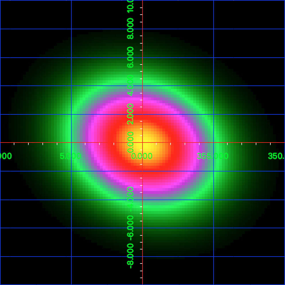
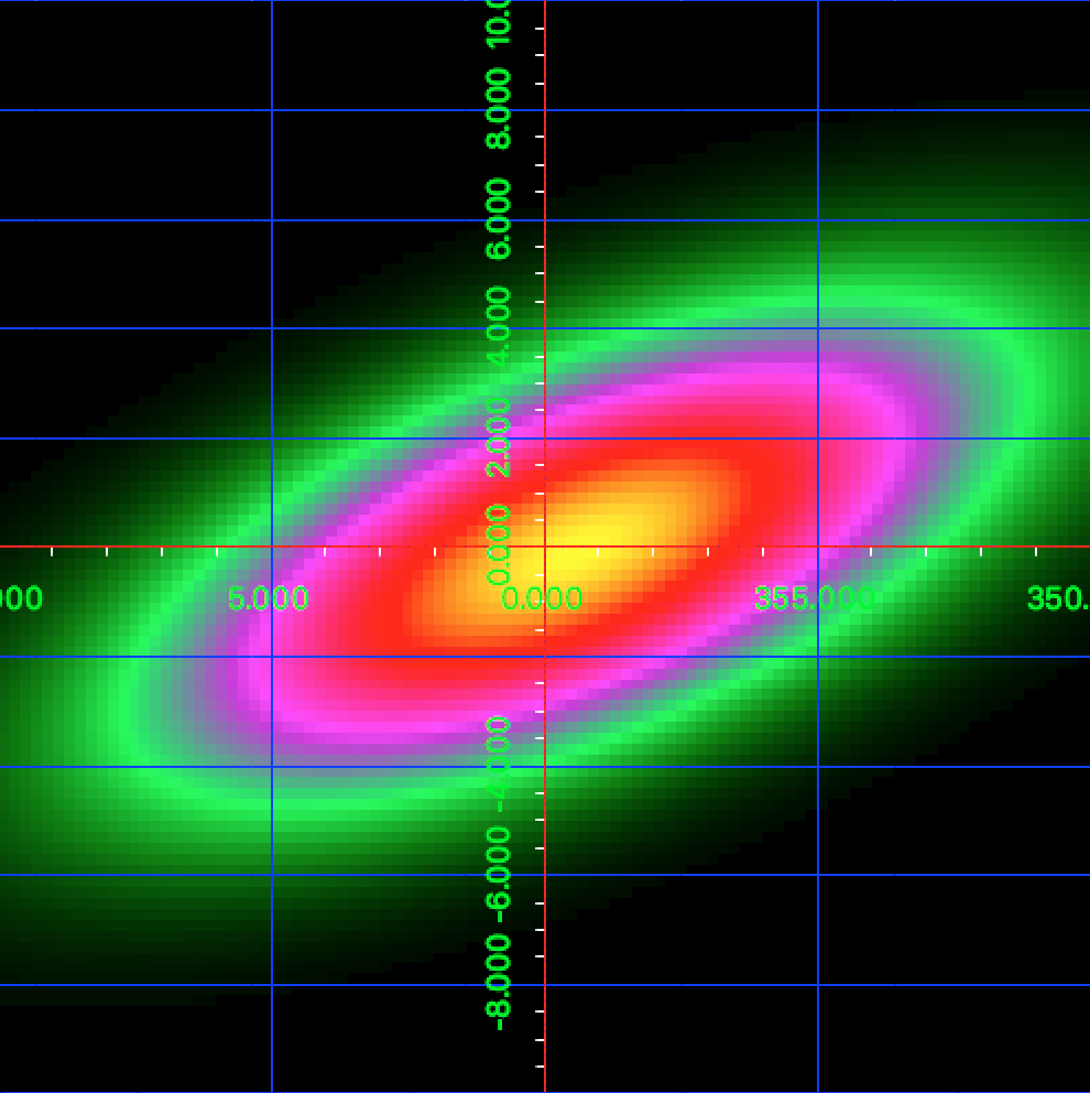
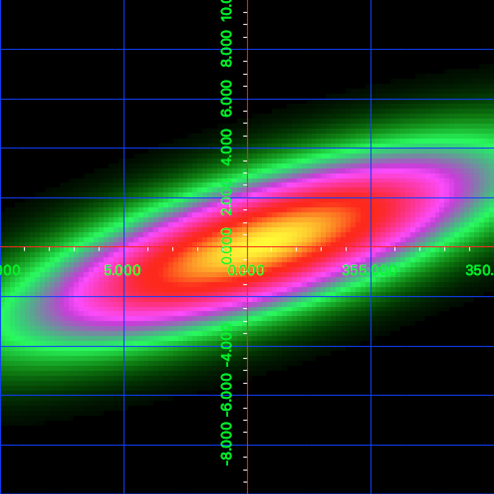
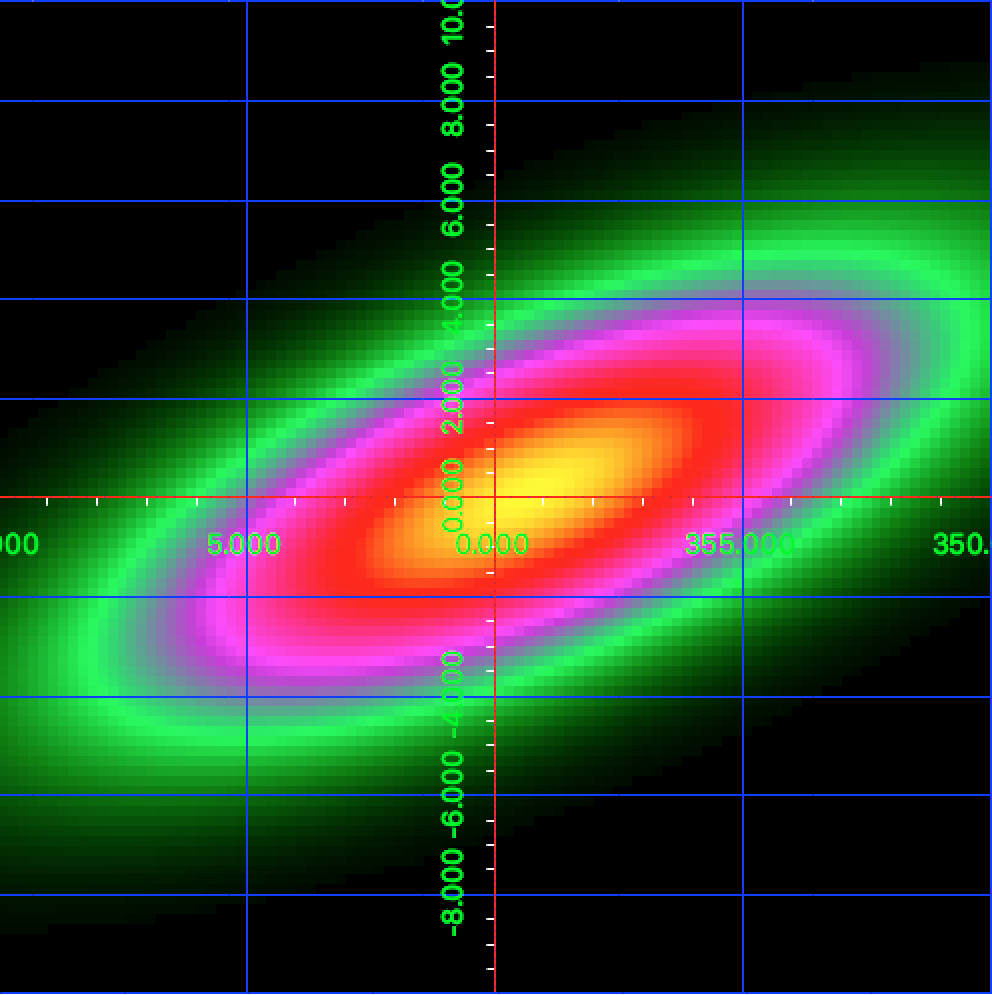
And here the results for an elliptical Gaussian model. As for the radial models, two parameters m_irf_elliptical_iter_theta and m_irf_elliptical_iter_phi were added to control the results. Also 6 integration iterations in both directions seem satisfactory. To illustrate the fitted ellipse sky images were generated in Galactic coordinates. They are shown below, with 4 iterations on the top left plot, 5 on the top right plot, 6 on the bottom left plot and 7 iterations at the top right.
| Theta | Phi | MLR | RA | DEC | PA | Major | Minor | Norm | CPU (s) |
| 4 | 4 | 494.704 | 266.43 +/- 0.18 | -29.07 +/ - 0.15 | 8.7 +/- 13.6 | 3.25 +/- 0.24 | 2.59 +/- 0.25 | 0.1397 +/- 0.0067 | 1347 |
| 5 | 5 | 518.144 | 265.96 +/- 0.27 | -29.36 +/ - 0.20 | 48.9 +/- 2.0 | 6.58 +/- 0.38 | 1.69 +/- 0.03 | 0.1741 +/- 0.0097 | 3871 |
| 6 | 6 | 513.506 | 266.13 +/- 0.43 | -29.48 +/ - 0.28 | 54.5 +/- 4.6 | 5.34 +/- 0.52 | 2.06 +/- 0.23 | 0.1549 +/- 0.0079 | 17260 |
| 7 | 7 | 515.771 | 265.91 +/- 0.47 | -29.49 +/ - 0.30 | 54.9 +/- 4.1 | 5.73 +/- 0.62 | 2.06 +/- 0.24 | 0.1578 +/- 0.0082 | 70180 |
 |
 |
 |
 |
#18
Updated by Knödlseder Jürgen almost 5 years ago
- File deleted (
elliptical_map_iter4-4.fits)
#19
Updated by Knödlseder Jürgen almost 5 years ago
- File deleted (
elliptical_map_iter5-5.fits)
#20
Updated by Knödlseder Jürgen almost 5 years ago
- File deleted (
elliptical_map_iter6-6.fits)
#21
Updated by Knödlseder Jürgen almost 5 years ago
- File deleted (
elliptical_map_iter7-7.fits)
#22
Updated by Knödlseder Jürgen almost 5 years ago
- File map_elliptical_iter4-4.png added
- File map_elliptical_iter5-5.png added
- File map_elliptical_iter6-6.png added
- File map_elliptical_iter7-7.png added
#23
Updated by Knödlseder Jürgen almost 5 years ago
- % Done changed from 70 to 100
Here a comparison of the diffuse model analysis. An extended Gaussian disk was fitted on top of the map disk-robin2003-d1.fits for the Galactic disk emission to the 511 keV data.
The table below compares the spi_obs_fit to the ctlike result. ctlike compares the MLR for each component, no computation of H0 is done. Yet from the analysis above the H0 value is known (in parentheses), resulting in a total MLR of 475.516, very close to the value obtained with spi_obs_fit. All other fit results are extremely close. The only significant difference is the computing time, which is about 170 times longer for ctlike compared to spi_obs_fit. This is related to the very inefficient GSPIResponse::irf_diffuse method
The ctlike fitting factor for the bulge is 0.20198 +/- 0.01346 ph/cm2/s/MeV. Since the fit was done for a band of 7 keV, the value has to be multiplied by the band width to give (141.4 +/- 9.4)e-05 (note that spi_obs_fit gives flux values in 1e-05 ph/cm2/s).
The ctlike fitting factor for the disk map is 0.17428 +/- 0.06190 ph/cm2/s/MeV. The total flux in the map is 4.2791e-04 ph/cm2/s/MeV, and ctlike divides the map internally by this value before model fitting. Hence the fitted map flux corresponds to (2.85 +/- 1.01)e-05 ph/cm2/s/MeV.
| Analysis | H1 | H0 | MLR | Bulge | Disk | CPU (s) |
| spi_obs_fit | -256643525.575 | -256643287.777 | 475.597 | 142.1 +/- 9.4 | 2.8 +/- 1.0 | 191.0 |
| ctlike | -256643525.535 | (-256643287.777) | (475.516) 266.405 / 7.934 | 141.4 +/- 9.4 | 2.9 +/- 1.0 | 32354.3 |
#24
Updated by Knödlseder Jürgen almost 5 years ago
- Status changed from In Progress to Pull request
The implementation of the GSPIResponse class is now finished, all computations previously possible with spi_toolslib are possible, and also the fitting of spatial parameters works.
#25
Updated by Knödlseder Jürgen almost 5 years ago
- Status changed from Pull request to Closed
Merged into devel.