Updated over 11 years ago by Knödlseder Jürgen

GCTAResponse¶

• GCTAResponse
  • Diffuse model response
    • GCTAResponse::irf_diffuse
    • GCTAResponse::npred_diffuse
    • Diffuse model testing
      • Diffuse model only
      • Diffuse and background model

Diffuse model response¶

The diffuse model response is implemented by the methods GCTAResponse::irf_diffuse and GCTAResponse::npred_diffuse.

GCTAResponse::irf_diffuse¶

GCTAResponse::irf_diffuse performs an integration over the true photon arrival direction of the sky map times the instrument response function. The integration is performed in the reference of the observed photon direction. The offset angle (or theta) integration is performed using the helper class cta_irf_diffuse_kern_theta while the azimuth angle (or phi) integration is performed using the helper class cta_irf_diffuse_kern_phi.

Some analysis has been done to estimate the required precision of the integration. For this purpose, a 180000 s observation of Cen A has been simulated using ctobssim, with a deadtime correction of 0.889. The ROI radius was set to 7.5 deg, the energy range spanned 0.1-100 TeV. The events were then subsequently binned using ctbin (100 bins of 0.05 times 0.05 deg). The number of events binned by gtbin was 1117428, hence the expected number of events for a integration time of 1800 s should be 11174.28.

Below are the model computation results for a 1800 s integration period and the same observation parameters as used for the simulations. The computation was performed using the test_response_irf function in the test_CTA.cpp file. As the test uses event binning, we also studied the impact of the number of energy bins on the result:

Theta	Phi	Ebins	Events	Uncertainty	Time
1e-4	1e-4	5	12387.8	+10.859%	1m7.4s
1e-4	1e-4	10	11325.4	+1.352%	2m49.1s
1e-4	1e-4	20	11219.2	+0.402%	5m24.1s
1e-4	1e-4	30	11207.3	+0.296%	8m46.6s
1e-3	1e-3	30	11207.4	+0.296%	3m5.0s
1e-2	1e-2	30	11207.2	+0.295%	1m43.1s
1e-1	1e-1	30	11207.2	+0.295%	1m41.9s

Obviously, there is a clear impact of the number of energy bins used on the precision of the model computation, so we stick to 30 energy bins for the evaluation of the integration precision.

It is interesting to notice that the uncertainty in the model computation is basically independent of the integration precision. This can be understood by the fact that the integration is done over the size of the PSF, and if the model and effective do not vary drastically over this size, the integration converges quickly.

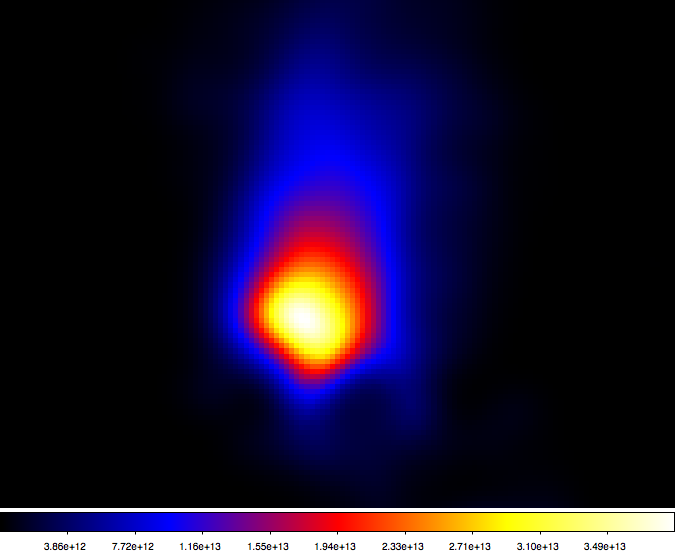
To illustrate that even with a low precision of 1e-2 and 1e-3 satisfactory images are obtained, model maps of the Cen A map are shown below. The FITS files of the model maps with all ten energy layers are attached to the page for reference.

Integration precision = 1e-2	Integration precision = 1e-3

For the moment (18/07/2012) we set the precisions to 1e-2 for the Phi and Theta integrations. Reducing the precision to an even smaller value does not seem to improve the performances.

GCTAResponse::npred_diffuse¶

GCTAResponse::npred_diffuse performs an integration of the sky map times the point source Npred method over the region of interest. The offset angle integration is performed using the helper class cta_npred_diffuse_kern_theta while the azimuth angle integration is performed using the helper class cta_npred_diffuse_kern_phi.

Some analysis has been done to estimate the required precision of the integration. For this purpose a 1800 s observation of Cen A has been simulated, with a deadtime correction of 0.889. The ROI radius was set to 5.0 deg, the energy range spanned 0.1-100 TeV. In doing 10 ctobssim runs, the mean/median number of simulated events was 11232/11239. Doing a single ctobssim run of 180000 s, the number of simulated events was 1124003. The expected number of events should thus be 11240.

Here now the results obtained from the Npred computation for the same observation parameters. The computation was performed using the test_response_npred function in the test_CTA.cpp file:

Theta	Phi	Events	Uncertainty	Time
1e-6	1e-6	11240.6	+0.005%	6m28s
1e-6	1e-4	11237.9	-0.019%	1m4.6s
1e-4	1e-4	11212.3	-0.246%	0m6.2s
1e-5	1e-5	11238.8	-0.011%	0m49.2s
5e-5	5e-5	11225.2	-0.132%	0m11.7s
1e-4	1e-5	11246.2	+0.055%	0m16.5s
1e-5	1e-4	11236.2	-0.034%	0m15.4s
1e-3	1e-3	11135.2	-0.932%	0m1.3s

For the moment (18/07/2012) we set the precisions to 1e-4 for the Phi and Theta integrations. Eventually, we may reduce them further to 1e-3, but we should first see how this globally affects the fit results.

Note that the integration over energy which is performed using the GObservation::npred_spec method uses a precision of 1e-6. Decreasing the precision down to 1e-5 results in an estimated number of 11239.4 events while reducing the computing time to 0m35s. We should think about reducing globally the precision of the Romberg integrator (to maybe 1e-5).

5/4/2013:
Here some fit results depending on precision. What is show is the fitted pre factor and index. The true pre factor was 1e-7, the true index was 2.100. The number of simulated Cen A events were 2414, the number of background events were 366, so the total number of events is 2780.

Theta	Phi	Prefactor	Index	Npred
1e-5	1e-5	0.442e-7 +/- 0.168e-7	2.067 +/- 0.037	2780
1e-4	1e-4	0.426e-7 +/- 0.162e-7	2.065 +/- 0.037	2780
1e-3	1e-3	0.448e-7 +/- 0.171e-7	2.070 +/- 0.037	2780

I also check the precision in GObservation::npred_spec:

npred_spec	Evaluations	Events		1e-6	128	11212.3
1e-5	64	11212.4
1e-4	32	11217.2
1e-3	16	11388.3

This indicates that (at least for a power law) a value of 1e-5 is okay.

Diffuse model testing¶

Diffuse model only¶

The implementation of the diffuse model response has been tested using a Cen A simulation. The integration time has been set to 1800 s using the default deadc of ctobssim. Events have been simulated for an acceptance cone of 7.5 deg around Cen A. The events spanned an energy range of 0.1-100 TeV. A total of 11956 events has been simulated. Using ctselect, events have then be selected within a radius of 5 deg. This resulted in 11956 events, i.e. the same number as simulated (apparently, the Cen A sky map is smaller than the 5 deg ROI).

The model used for the simulation was the following:

<?xml version="1.0" standalone="no"?>
<source_library title="source library">
    <source name="Cen A lobes" type="DiffuseSource">
    <spectrum type="PowerLaw">
        <parameter scale="1e-07" name="Prefactor" min="1e-07" max="1000.0" value="1.73" free="1"/>
        <parameter scale="1.0" name="Index" min="-5.0" max="+5.0" value="-2.1" free="1"/>
        <parameter scale="1.0" name="Scale" min="10.0" max="1000000.0" value="100.0" free="0"/>
    </spectrum>
    <spatialModel type="SpatialMap" file="data/cena_lobes_parkes.fits">
        <parameter scale="1" name="Prefactor" min="0.001" max="1000.0" value="1" free="0"/>
    </spatialModel>
    </source>
</source_library>

Using ctlike, the following results have been obtained:

2012-07-18T12:55:14: === GOptimizerLM ===
2012-07-18T12:55:14:  Optimized function value ..: 93564.5
2012-07-18T12:55:14:  Absolute precision ........: 1e-06
2012-07-18T12:55:14:  Optimization status .......: converged
2012-07-18T12:55:14:  Number of parameters ......: 5
2012-07-18T12:55:14:  Number of free parameters .: 2
2012-07-18T12:55:14:  Number of iterations ......: 3
2012-07-18T12:55:14:  Lambda ....................: 1e-06
2012-07-18T12:55:14:  Maximum log likelihood ....: -93564.5
2012-07-18T12:55:14:  Npred .....................: 11956
2012-07-18T12:55:14: === GModels ===
2012-07-18T12:55:14:  Number of models ..........: 1
2012-07-18T12:55:14:  Number of parameters ......: 5
2012-07-18T12:55:14: === GModelDiffuseSource ===
2012-07-18T12:55:14:  Name ......................: Cen A lobes
2012-07-18T12:55:14:  Instruments ...............: all
2012-07-18T12:55:14:  Model type ................: "SpatialMap" * "PowerLaw" * "Constant" 
2012-07-18T12:55:14:  Number of parameters ......: 5
2012-07-18T12:55:14:  Number of spatial par's ...: 1
2012-07-18T12:55:14:   Prefactor ................: 1 [0.001,1000]  (fixed,scale=1,gradient)
2012-07-18T12:55:14:  Number of spectral par's ..: 3
2012-07-18T12:55:14:   Prefactor ................: 1.8199e-07 +/- 9.56868e-09 [1e-14,0.0001] ph/cm2/s/MeV (free,scale=1e-07,gradient)
2012-07-18T12:55:14:   Index ....................: -2.10617 +/- 0.00565118 [-5,5]  (free,scale=1,gradient)
2012-07-18T12:55:14:   PivotEnergy ..............: 100 [10,1e+06] MeV (fixed,scale=1,gradient)
2012-07-18T12:55:14:  Number of temporal par's ..: 1
2012-07-18T12:55:14:   Constant .................: 1 (relative value) (fixed,scale=1,gradient)

As expected for a good fit, Npred is equal to the observed number of events. The Prefactor is at +0.94 sigma above the true value, the index is at -1.09 sigma below the true value. This offset is reasonable.

As next step the events have been binned using ctbin (30 energy slices from 0.1-100 TeV, 100 x 100 pixels with binsize of 0.05 pixels). This resulted in 11884 events binned into the counts map. ctlike was then employed to fit the counts map. The following results have been obtained:

2012-07-18T13:14:15: === GOptimizerLM ===
2012-07-18T13:14:15:  Optimized function value ..: 24976.5
2012-07-18T13:14:15:  Absolute precision ........: 1e-06
2012-07-18T13:14:15:  Optimization status .......: converged
2012-07-18T13:14:15:  Number of parameters ......: 5
2012-07-18T13:14:15:  Number of free parameters .: 2
2012-07-18T13:14:15:  Number of iterations ......: 3
2012-07-18T13:14:15:  Lambda ....................: 1e-06
2012-07-18T13:14:15:  Maximum log likelihood ....: -24976.5
2012-07-18T13:14:15:  Npred .....................: 11884
2012-07-18T13:14:15: === GModels ===
2012-07-18T13:14:15:  Number of models ..........: 1
2012-07-18T13:14:15:  Number of parameters ......: 5
2012-07-18T13:14:15: === GModelDiffuseSource ===
2012-07-18T13:14:15:  Name ......................: Cen A lobes
2012-07-18T13:14:15:  Instruments ...............: all
2012-07-18T13:14:15:  Model type ................: "SpatialMap" * "PowerLaw" * "Constant" 
2012-07-18T13:14:15:  Number of parameters ......: 5
2012-07-18T13:14:15:  Number of spatial par's ...: 1
2012-07-18T13:14:15:   Prefactor ................: 1 [0.001,1000]  (fixed,scale=1,gradient)
2012-07-18T13:14:15:  Number of spectral par's ..: 3
2012-07-18T13:14:15:   Prefactor ................: 1.82128e-07 +/- 9.61141e-09 [1e-14,0.0001] ph/cm2/s/MeV (free,scale=1e-07,gradient)
2012-07-18T13:14:15:   Index ....................: -2.10646 +/- 0.0056721 [-5,5]  (free,scale=1,gradient)
2012-07-18T13:14:15:   PivotEnergy ..............: 100 [10,1e+06] MeV (fixed,scale=1,gradient)
2012-07-18T13:14:15:  Number of temporal par's ..: 1
2012-07-18T13:14:15:   Constant .................: 1 (relative value) (fixed,scale=1,gradient)

Again, Npred is equal to the observed number of events. The Prefactor and index are very similar (but not identical) to the results obtained using an unbinned analysis.

Diffuse and background model¶

Now I fitted a diffuse model on top of the background model. The XML file used for the model is shown below:

<?xml version="1.0" standalone="no"?>
<source_library title="source library">
  <source name="Cen A lobes" type="DiffuseSource">
    <spectrum type="PowerLaw">
       <parameter name="Prefactor" scale="1e-16" value="5.7"  min="1e-07" max="1000.0" free="1"/>
       <parameter name="Index"     scale="-1"    value="2.48" min="0.0"   max="+5.0"   free="1"/>
       <parameter name="Scale"     scale="1e6"   value="0.3"  min="0.01"  max="1000.0" free="0"/>
    </spectrum>
    <spatialModel type="SpatialMap" file="data/cena_lobes_parkes.fits">
        <parameter scale="1" name="Prefactor" min="0.001" max="1000.0" value="1" free="0"/>
    </spatialModel>
    </source>
  <source name="Background" type="RadialAcceptance" instrument="CTA">
    <spectrum type="PowerLaw">
       <parameter name="Prefactor" scale="1e-6" value="61.8" min="0.0"  max="1000.0" free="1"/>
       <parameter name="Index"     scale="-1"   value="1.85" min="0.0"  max="+5.0"   free="1"/>
       <parameter name="Scale"     scale="1e6"  value="1.0"  min="0.01" max="1000.0" free="0"/>
    </spectrum>
    <radialModel type="Gaussian">
       <parameter name="Sigma" scale="1.0" value="3.0" min="0.01" max="10.0" free="1"/>
    </radialModel>
  </source>
</source_library>

There were 581 counts for Cen A and 3250 counts in the background, giving a total of 3831 counts. The ctselect step left again the total number of counts unchanged. The (unbinned) ctlike run gave the following result:

2012-07-18T13:31:51: === GOptimizerLM ===
2012-07-18T13:31:51:  Optimized function value ..: 34312.9
2012-07-18T13:31:51:  Absolute precision ........: 1e-06
2012-07-18T13:31:51:  Optimization status .......: converged
2012-07-18T13:31:51:  Number of parameters ......: 10
2012-07-18T13:31:51:  Number of free parameters .: 5
2012-07-18T13:31:51:  Number of iterations ......: 4
2012-07-18T13:31:51:  Lambda ....................: 1e-07
2012-07-18T13:31:51:  Maximum log likelihood ....: -34312.9
2012-07-18T13:31:51:  Npred .....................: 3831
2012-07-18T13:31:51: === GModels ===
2012-07-18T13:31:51:  Number of models ..........: 2
2012-07-18T13:31:51:  Number of parameters ......: 10
2012-07-18T13:31:51: === GModelDiffuseSource ===
2012-07-18T13:31:51:  Name ......................: Cen A lobes
2012-07-18T13:31:51:  Instruments ...............: all
2012-07-18T13:31:51:  Model type ................: "SpatialMap" * "PowerLaw" * "Constant" 
2012-07-18T13:31:51:  Number of parameters ......: 5
2012-07-18T13:31:51:  Number of spatial par's ...: 1
2012-07-18T13:31:51:   Prefactor ................: 1 [0.001,1000]  (fixed,scale=1,gradient)
2012-07-18T13:31:51:  Number of spectral par's ..: 3
2012-07-18T13:31:51:   Prefactor ................: 5.49351e-16 +/- 4.03622e-17 [1e-23,1e-13] ph/cm2/s/MeV (free,scale=1e-16,gradient)
2012-07-18T13:31:51:   Index ....................: -2.52938 +/- 0.0527701 [-0,-5]  (free,scale=-1,gradient)
2012-07-18T13:31:51:   PivotEnergy ..............: 300000 [10000,1e+09] MeV (fixed,scale=1e+06,gradient)
2012-07-18T13:31:51:  Number of temporal par's ..: 1
2012-07-18T13:31:51:   Constant .................: 1 (relative value) (fixed,scale=1,gradient)
2012-07-18T13:31:51: === GCTAModelRadialAcceptance ===
2012-07-18T13:31:51:  Name ......................: Background
2012-07-18T13:31:51:  Instruments ...............: CTA
2012-07-18T13:31:51:  Model type ................: "Gaussian" * "PowerLaw" * "Constant" 
2012-07-18T13:31:51:  Number of parameters ......: 5
2012-07-18T13:31:51:  Number of radial par's ....: 1
2012-07-18T13:31:51:   Sigma ....................: 3.00231 +/- 0.0376892 [0.01,10] deg2 (free,scale=1,gradient)
2012-07-18T13:31:51:  Number of spectral par's ..: 3
2012-07-18T13:31:51:   Prefactor ................: 6.56254e-05 +/- 2.06902e-06 [0,0.001] ph/cm2/s/MeV (free,scale=1e-06,gradient)
2012-07-18T13:31:51:   Index ....................: -1.82475 +/- 0.017447 [-0,-5]  (free,scale=-1,gradient)
2012-07-18T13:31:51:   PivotEnergy ..............: 1e+06 [10000,1e+09] MeV (fixed,scale=1e+06,gradient)
2012-07-18T13:31:51:  Number of temporal par's ..: 1
2012-07-18T13:31:51:   Constant .................: 1 (relative value) (fixed,scale=1,gradient)

Also here, Npred corresponds to the observed number of counts. The prefactor is at -0.51 sigma and the index is at -0.94 sigma from the expected model values, which is pretty reasonable.