Updated almost 11 years ago by Schulz Anneli
- Validation of Pass 7Rep data
Validation of Pass 7Rep data
The versions of the software are: Science Tools 09-32-05 and ctools (devel from 08.01.14)
Cross check 1: 1 week Fermi LAT data, crab region (Anneli)
Using the following parameters:
ra = 83.6331
dec = 22.0145

rad = 7.5deg,
map: 10x10 deg, 0.1 degperbin
zmax = 100
emin = 100 MeV
emax = 10000 MeV

tmin = 239557446.6 MET in s
tmax= 240162199.6 MET in s
nebins = 20
I performed a standard Fermi analysis and in the end performed a gtlike fit. The data files ( srcmap, exposure cube and ltcube) are produced within the Fermi Science Tools and are the same for gtlike and ctlike.
The model used to describe the data contains only the Crab as a Point Source with a power-law2 spectral model and the galactic and isotropic diffuse models.
| Parameter | gtlike | ctlike |
| Crab integral flux [1e-7] | 25.59 +/- 1.51 | 19.92 +/- 1.19 |
| Crab index | - 2.135 +/- 0.0460 | - 2.051 +/- 0.049 |
| Gal prefac | 0.729 +/- 0.144 | 0.774+/- 0.157 |
| Gal index | 0.087 +/- 0.072 | 0.070 +/- 0.074 |
| Iso normalization | 2.876 +/- 0.686 | 3.486 +/- 0.694 |
The same dataset with the index fixed:
| Parameter | gtlike | ctlike |
| Crab integral flux [1e-7] | 24.87 +/- 1.17 | 20.62 +/- 0.99 |
| Crab index | - 2.1 | - 2.1 |
| Gal prefac | 0.721 +/- 0.145 | 0.783 +/- 0.155 |
| Gal index | 0.085 +/- 0.072 | 0.071 +/- 0.073 |
| Iso normalization | 3.033 +/- 0.657 | 3.326 +/- 0.674 |
the same dataset with the diffuse models fixed:
| Parameter | gtlike | ctlike | |
Crab integral flux [1e-9] | 32.99 +/- 2.29 | 26.35 +/- 1.91 |
| Crab index | - 2.186 +/- 0.041 | - 2.136 +/- 0.042 | ||||
| Gal prefac | 1 | 1 | ||||
| Gal index | 0 | 0 | ||||
| Iso normalization | 1 | 1 | ||||
| nobs | 2225 | 2225 | |
npred | 2193 | 2107.66 |
| log L | 10812 | 10839.8 |
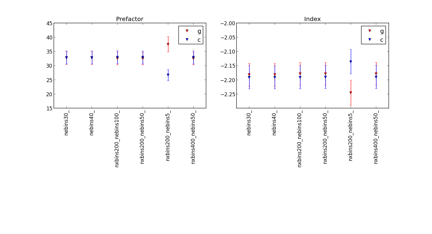
Plot showing the differences for different numbers of energy bins
before the fix: 
after Jürgen’s fix: 
showing that the fit results are quite similar, but be carful to use enough energy bins.
Updated table
diffuse sources also free during fit :| Parameter | gtlike | ctlike after fix | ctlike before fix |
| Crab integral flux [1e-7] | 25.59 +/- 1.51 | 25.25 +/- 1.51 | 19.92 +/- 1.19 |
| Crab index | - 2.135 +/- 0.0460 | - 2.137+/- 0.048 | - 2.051 +/- 0.049 |
| Gal prefac | 0.729 +/- 0.144 | 0.728 +/- 0.151 | 0.774+/- 0.157 |
| Gal index | 0.087 +/- 0.072 | 0.078 +/- 0.076 | 0.070 +/- 0.074 |
| Iso normalization | 2.876 +/- 0.686 | 2.912 +/- 0.692 | 3.486 +/- 0.694 |
Jürgen’s analysis
I also started to investigate the P7REP data/response. For that purpose I create a 20°x20° binned dataset for the first mission week using the P7REP_SOURCE_V15 response. The log file for building the dataset is here: log.txt. The dataset spans 20 logarithmically spaced energy bins from 200 MeV to 20 GeV. I used ScienceTools-09-32-05 and gammalib-00-08-02 / ctools-00-07-02 (10/2/2014).
gtlike reference result
The gtlike run gives the following results:
<===> Crab:
<===> Integral: 23.7269 +/- 1.75163
<===> Index: -2.13911 +/- 0.05222
<===> LowerLimit: 100
<===> UpperLimit: 500000
<===> TS value: 1420.34
<===> Flux: 1.07194e-06 +/- 5.77353e-08 photons/cm^2/s
<===>
<===> Extragal_diffuse:
<===> Normalization: 1.36172 +/- 0.358261
<===> Flux: 9.47324e-05 +/- 2.49144e-05 photons/cm^2/s
<===>
<===> Galactic_diffuse:
<===> Value: 1.11336 +/- 0.040282
<===> MapBase::readFitsFile: creating WcsMap2 object
<===> Flux: 0.000332391 +/- 1.20257e-05 photons/cm^2/s
<===> WARNING: Fit may be bad in range [3169.79, 3990.52] (MeV)
<===>
<===>
<===> Total number of observed counts: 4832
<===> Total number of model events: 4832.12
<===> 114  -25979.56744  4832.121898
<===>
<===> -log(Likelihood): 25979.56744
ctlike reference result
The ctlike run gives the following result:
2014-02-10T22:51:21: === GOptimizerLM ===
2014-02-10T22:51:21:  Optimized function value ..: 25988.630
2014-02-10T22:51:21:  Absolute precision ........: 1e-06
2014-02-10T22:51:21:  Optimization status .......: converged
2014-02-10T22:51:21:  Number of parameters ......: 13
2014-02-10T22:51:21:  Number of free parameters .: 4
2014-02-10T22:51:21:  Number of iterations ......: 10
2014-02-10T22:51:21:  Lambda ....................: 1e-13
2014-02-10T22:51:21:  Maximum log likelihood ....: -25988.630
2014-02-10T22:51:21:  Observed events  (Nobs) ...: 4832.000
2014-02-10T22:51:21:  Predicted events (Npred) ..: 4832.000 (Nobs - Npred = 2.56947e-06)
2014-02-10T22:51:21: === GModels ===
2014-02-10T22:51:21:  Number of models ..........: 3
2014-02-10T22:51:21:  Number of parameters ......: 13
2014-02-10T22:51:21: === GModelSky ===
2014-02-10T22:51:21:  Name ......................: Extragal_diffuse
2014-02-10T22:51:21:  Instruments ...............: all
2014-02-10T22:51:21:  Instrument scale factors ..: unity
2014-02-10T22:51:21:  Observation identifiers ...: all
2014-02-10T22:51:21:  Model type ................: DiffuseSource
2014-02-10T22:51:21:  Model components ..........: "ConstantValue" * "FileFunction" * "Constant"
2014-02-10T22:51:21:  Number of parameters ......: 3
2014-02-10T22:51:21:  Number of spatial par's ...: 1
2014-02-10T22:51:21:   Value ....................: 1 [0,10]  (fixed,scale=1,gradient)
2014-02-10T22:51:21:  Number of spectral par's ..: 1
2014-02-10T22:51:21:   Normalization ............: 1.54418 +/- 0.351893 [0,1000]  (free,scale=1,gradient)
2014-02-10T22:51:21:  Number of temporal par's ..: 1
2014-02-10T22:51:21:   Constant .................: 1 (relative value) (fixed,scale=1,gradient)
2014-02-10T22:51:21: === GModelSky ===
2014-02-10T22:51:21:  Name ......................: Galactic_diffuse
2014-02-10T22:51:21:  Instruments ...............: all
2014-02-10T22:51:21:  Instrument scale factors ..: unity
2014-02-10T22:51:21:  Observation identifiers ...: all
2014-02-10T22:51:21:  Model type ................: DiffuseSource
2014-02-10T22:51:21:  Model components ..........: "MapCubeFunction" * "ConstantValue" * "Constant"
2014-02-10T22:51:21:  Number of parameters ......: 3
2014-02-10T22:51:21:  Number of spatial par's ...: 1
2014-02-10T22:51:21:   Normalization ............: 1 [0.001,1000]  (fixed,scale=1,gradient)
2014-02-10T22:51:21:  Number of spectral par's ..: 1
2014-02-10T22:51:21:   Value ....................: 1.09883 +/- 0.0391273 [0,1000]  (free,scale=1,gradient)
2014-02-10T22:51:21:  Number of temporal par's ..: 1
2014-02-10T22:51:21:   Constant .................: 1 (relative value) (fixed,scale=1,gradient)
2014-02-10T22:51:21: === GModelSky ===
2014-02-10T22:51:21:  Name ......................: Crab
2014-02-10T22:51:21:  Instruments ...............: all
2014-02-10T22:51:21:  Instrument scale factors ..: unity
2014-02-10T22:51:21:  Observation identifiers ...: all
2014-02-10T22:51:21:  Model type ................: PointSource
2014-02-10T22:51:21:  Model components ..........: "SkyDirFunction" * "PowerLaw2" * "Constant"
2014-02-10T22:51:21:  Number of parameters ......: 7
2014-02-10T22:51:21:  Number of spatial par's ...: 2
2014-02-10T22:51:21:   RA .......................: 83.6331 [-360,360] deg (fixed,scale=1)
2014-02-10T22:51:21:   DEC ......................: 22.0145 [-90,90] deg (fixed,scale=1)
2014-02-10T22:51:21:  Number of spectral par's ..: 4
2014-02-10T22:51:21:   Integral .................: 2.03031e-06 +/- 1.62742e-07 [1e-14,0.0001] ph/cm2/s (free,scale=1e-07,gradient)
2014-02-10T22:51:21:   Index ....................: -2.09525 +/- 0.06069 [-5,5]  (free,scale=1,gradient)
2014-02-10T22:51:21:   LowerLimit ...............: 100 [10,1e+06] MeV (fixed,scale=1)
2014-02-10T22:51:21:   UpperLimit ...............: 500000 [10,1e+06] MeV (fixed,scale=1)
2014-02-10T22:51:21:  Number of temporal par's ..: 1
2014-02-10T22:51:21:   Constant .................: 1 (relative value) (fixed,scale=1,gradient)
Fit result comparison
The following table compares the fit results:| Parameter | gtlike | ctlike |
| logL | -25979.567 | -25988.630 |
| Fitted counts | 4832.12 | 4832.000 |
| Crab Integral [1e-7] | 23.73 +/- 1.75 | 20.30 +/- 1.63 |
| Crab Index | - 2.14 +/- 0.05 | - 2.10 +/- 0.06 |
| Galactic diffuse | 1.11 +/- 0.04 | 1.10 +/- 0.04 |
| Isotropic | 1.36 +/- 0.36 | 1.54 +/- 0.35 |
The gtlike fit is a little better than the ctlike fit in terms of log likelihood.
Assessment of model counts in components
The number of counts attributed to the various model components has been determined by running gtlike and ctlike on models containing only the individual model components (for an example, see crab_model.xml; note that gtlike requires some fitting, hence the parameters were free’d within tiny limits around a fixed value). The ctlike run was done using obs_binned.xml. Here the results for the components:
| Component | gtlike logL | gtlike counts | ctlike logL | ctlike counts | gtlike-ctlike counts |
| Crab | -47611.137 | 595.886 | -52867.290 | 586.573 | 9.313 (-1.6%) |
| Isotropic | -35445.565 | 347.113 | -35458.969 | 347.562 | -0.449 (-0.1%) |
| Galactic | -26978.496 | 3380.41 | -26957.335 | 3434.584 | -54.174 (-1.6%) |
| All | -25979.567 | 4832.13 | -25991.482 | 4883.738 | -51.608 (-1.1%) |
The last line shows the results for fitting all components (with parameters held fixed at the optimum gtlike values).
Globally, gtlike and ctlike give within about 2% the same number of counts. Also the likelihoods are comparable (except for the Crab component; the difference is probably related to the different ways of treating zero counts in a model). Hence the response computation looks okay.
The fact that ctlike finds different parameters compared to gtlike seem to relate to a global mix between the model components that is different.
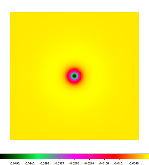
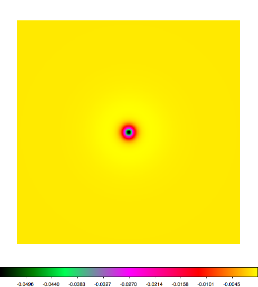
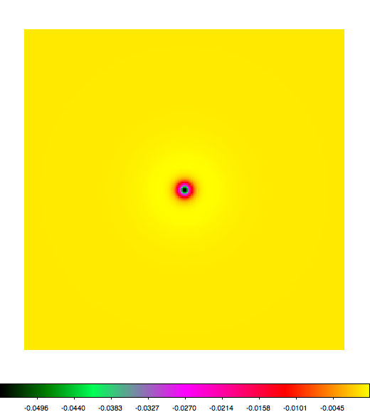
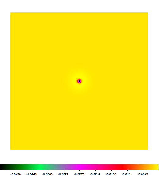
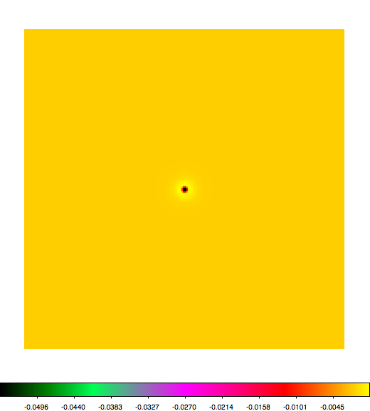
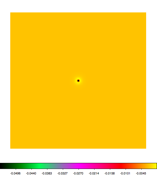
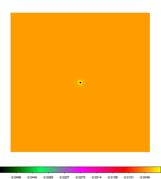
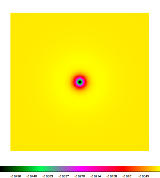
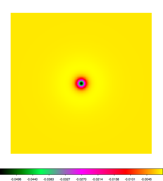
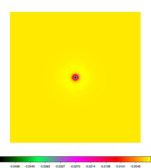
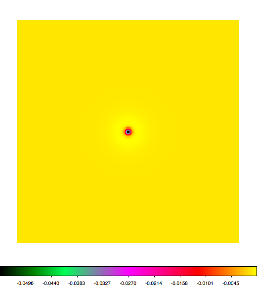
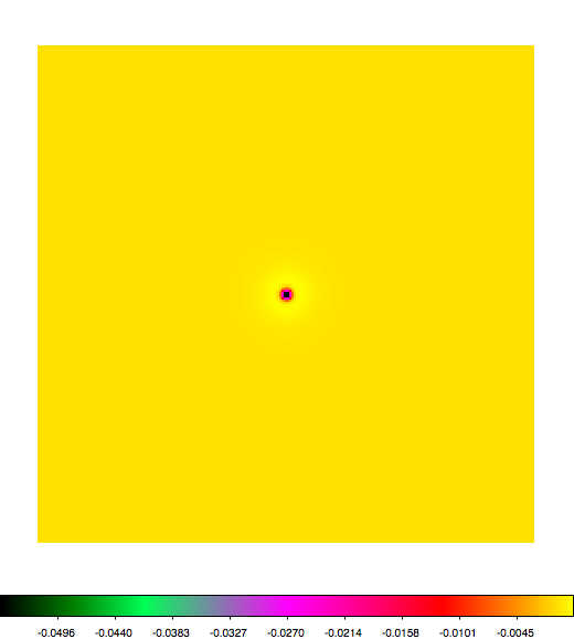
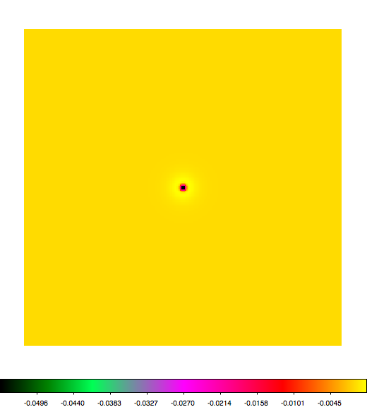
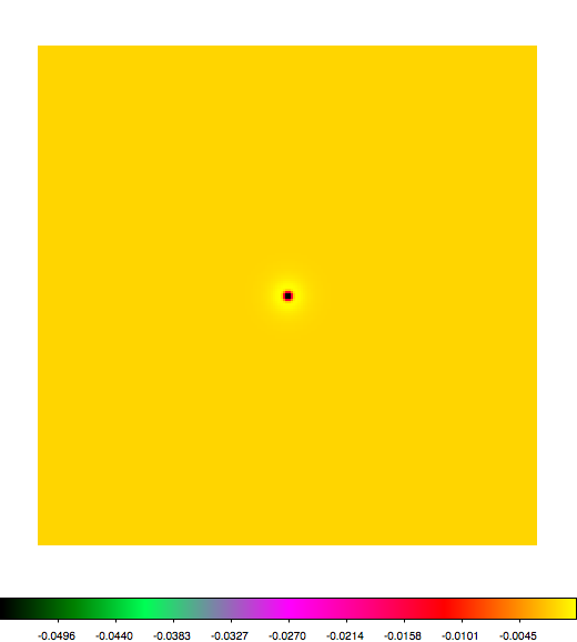
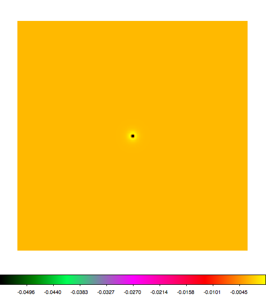
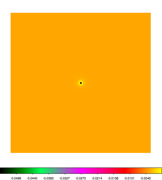
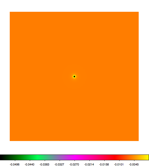
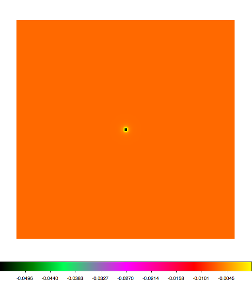
Below a mosaic of model differences for the Crab between Fermi Science Tools and gammalib. The differences are computed for a given source intensity (see crab_model.xml). The Fermi Science Tools model was computed using gtmodel, the gammalib model using lsmodel (a new cscript that I wrote for this purpose, ls means LAT script). gtmodel predicts 595.886 counts, lsmodel 586.573 counts. Images are from first energy bin to last energy (top left to bottom right).
 |
 |
 |
 |
 |
 |
 |
 |
 |
 |
 |
 |
 |
 |
 |
 |
 |
 |
 |
 |
A negative residual appears at the position of the Crab, meaning that gammalib predicts more counts at the core of the PSF with respect to the Fermi Science Tools. Conversely, the outer areas in the difference map are positive, indicating that gammalib predicts less counts in the tails of the PSF with respect to the Fermi Science Tools. This picture does not change when each energy bin of the cube is renormalized so that the gammalib and Fermi Science Tools cubes contain the same number of bins. Note that gtmodel has been run using
resample,b,h,yes,,,"Resample input counts map for convolution"
rfactor,i,h,2,,,"Resampling factor"
but the situation is the same when
resample=no is used.
Changing the zenith angle range
While comparing the ScienceTools to gammalib, I recognised that there was a small difference in the zenith angle range used. GammaLib was constrained to 70° in the GLATMeanPsf class, while in the Fermi/LAT ScienceTools went to the lower boundary of the response array (costheta=0.2). I changed this and verified that both softwares give the same exposure. Below the fit results before and after that change:
| Parameter | gtlike | ctlike before | ctlike after |
| logL | -25979.567 | -25988.630 | -25988.009 |
| Fitted counts | 4832.12 | 4832.000 | 4832.000 |
| Crab Integral [1e-7] | 23.73 +/- 1.75 | 20.30 +/- 1.63 | 20.07 +/- 1.61 |
| Crab Index | - 2.14 +/- 0.05 | - 2.10 +/- 0.06 | - 2.10 +/- 0.06 |
| Galactic diffuse | 1.11 +/- 0.04 | 1.10 +/- 0.04 | 1.10 +/- 0.04 |
| Isotropic | 1.36 +/- 0.36 | 1.54 +/- 0.35 | 1.54 +/- 0.35 |
The impact on the fit results is negligible.
Correcting scaling of back PSF
It turned out that the energy scaling of the back response was not correct! In fact, the code used the scaling of the front response for the back response, which resulted in incorrect PSF values for back. After fixing this problem, the following fit results are obtained (“ctlike before” refers to the same values given in the above table, hence before the costheta limit change):
| Parameter | gtlike | ctlike before | ctlike after |
| logL | -25979.567 | -25988.630 | -25980.191 |
| Fitted counts | 4832.12 | 4832.000 | 4832.000 |
| Crab Integral [1e-7] | 23.73 +/- 1.75 | 20.30 +/- 1.63 | 23.56 +/- 1.86 |
| Crab Index | - 2.14 +/- 0.05 | - 2.10 +/- 0.06 | - 2.14 +/- 0.06 |
| Galactic diffuse | 1.11 +/- 0.04 | 1.10 +/- 0.04 | 1.09 +/- 0.04 |
| Isotropic | 1.36 +/- 0.36 | 1.54 +/- 0.35 | 1.44 +/- 0.35 |
This obviously fixed the problem. Now the fit results for the Crab are pretty comparable.
Cross check 2: taking more data (now 5years of fermi data are available)
I started working on a larger data set and encountered some differences: one is documented in this issue [[https://cta-redmine.irap.omp.eu/issues/1150]]: , since I first thought that it might be a problem of special spectral models.
I started with an analysis of large dataset (5 years) in a ROI around W49B, which is close to the galactic plane, I have a large number of events:
Observed events (Nobs) ...: 1057409.000
this I fit in science tools ( including the models for 2FGL sources) and get reasonable values for the source and also the diffuse components and the other sources. ( too many numbers to put here)
Now to the cross-check with ctools:
Model from Fermi Science Tools: including many sources but fixed to fitted values
In the beginning I fixed all the sources (except the source of interest) to the fitted values a reanalysed it with ctools.
There the discrepancy between ctools (first value) compared to science tools (second value) is huge:
W49B
parameter: norm with value 0.000367931 compared to 0.00605515974
parameter: alpha with value 0.258841 compared to 2.275627162
parameter: beta with value 0.466763 compared to 0.05265050255
parameter: Eb with value 1880.54 compared to 1880.536653
I fixed the Eb to the value from the gtlike fit, since ctools are known to have a problem with correlated parameters (and Eb and norm are in this case). Free Eb makes the result even worse.
The norm of the fitted source is always close to the minimum. So I decided to go for “easier” model and do some checks:
Model from Fermi Science Tools:
including many sources but fixed to fitted values and only power law, powerlaw2 spectral models.
the second idea was that the reason might be the evaluation of of the PowerLaw with super exponential cutoff or log parabola, since both gave even worse results. But performing several checks I decided to go even a level lower and include only diffuse models in the ctools fit:
Assuming as a basis only the two diffuse models:
The values for the models are ( fitted in gtlike and fixed then in ctlike):
gal:
 Prefactor ................: 1.06256 [1e-05,100] ph/cm2/s/MeV (fixed,scale=1,gradient)
 Index ....................: -0.00511337 [-1,1]  (fixed,scale=1,gradient)
PivotEnergy ..............: 100 [50,2000] MeV (fixed,scale=1,gradient)
iso:
Normalization ............: 0.356774 [0,10]  (fixed,scale=1,gradient)
the number of predicted events in science tools is: 948640 while the number in ctools ( putting the models with fixed values in) is: 958766.087
This discrepancy of 10000 events might lead to wrong fitting results of the sources, which have much lower number of events.
Jürgen:
This is indeed strange. I looked into the srcmap file you sent and found one strange thing: the first and last layer of the isotropic diffuse component look pretty different in comparison to the other layers. For example, the first layer goes from 180174-379102 in value, about a factor 2 in range. The second layer runs from 376238-402911, a much more narrow dynamic range. I won’t expect that the response changes so quickly in energy. The before last layer covers 394973-428132 in range, the last layer covers 336460-409524. So somehow the first and last layers are different. I check with another srcmap file I have a I see not such a strange effect. Can you check the srcmap file and make sure that everything went well in creating the file?
By the way: I note that the predicted events from the ScienceTools (948640) is pretty off the observed number of events (1057409). When I fit the galactic diffuse and isotropic background using ctlike I get exactly the observed number of events and the following fit results:
gal:
Prefactor ................: 1.25116 +/- 0.00438167 [1e-05,100] ph/cm2/s/MeV (free,scale=1,gradient)
Index ....................: -0.0285025 +/- 0.00138844 [-1,1]  (free,scale=1,gradient)
PivotEnergy ..............: 100 [50,2000] MeV (fixed,scale=1,gradient)
iso:
Normalization ............: 0 +/- 0.038531 [0,10]  (free,scale=1,gradient)
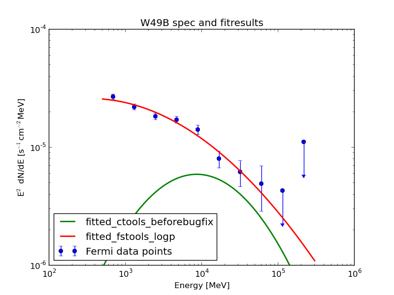
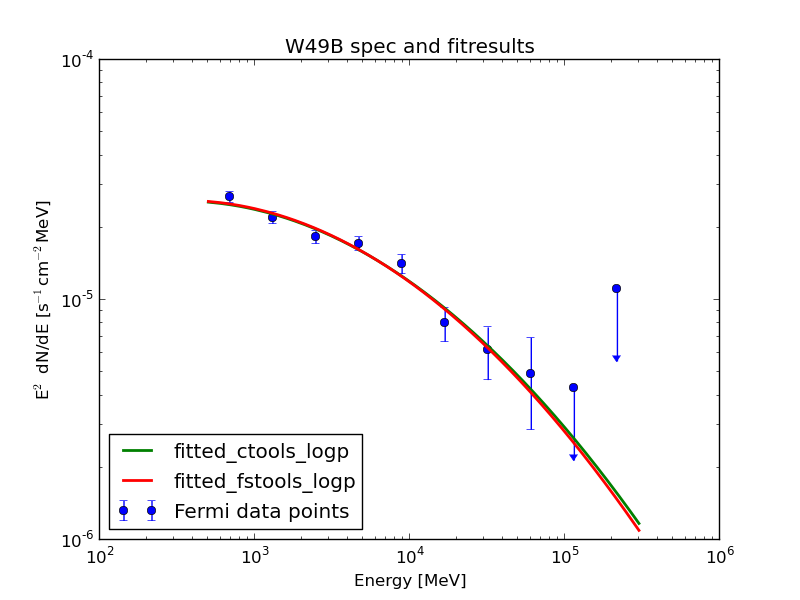
The fit pushes the isotropic component to zero. After Jürgen found a bug and fixed it (as described in https://cta-redmine.irap.omp.eu/issues/1004) everything looks quite promising: this plot shows the data points from science tools and the fit of science tools and ctools.
| Analysis | Norm@300MeV | Index | Curvature |
| ctools | 2.86 ± 0.04 | 1.99 ± 0.13 | 0.06 ± 0.03 |
| FSTs | 2.87 ± 0.02 | 1.98 ± 0.03 | 0.07 ± 0.01 |


log.txt  (24.9 KB)
crab_model.xml
(795 Bytes)
obs_binned.xml
(377 Bytes)
diff_bin_1.png (36.9 KB)
diff_bin_2.png (31.6 KB)
diff_bin_3.png (27.8 KB)
diff_bin_4.png (24.9 KB)
diff_bin_5.png (22.1 KB)
diff_bin_6.png (17 KB)
diff_bin_7.png (16.7 KB)
diff_bin_8.png (13.9 KB)
diff_bin_9.png (12.1 KB)
diff_bin_10.png (11.4 KB)
diff_bin_11.png (10.9 KB)
diff_bin_12.png (10 KB)
diff_bin_13.png (9.88 KB)
diff_bin_14.png (9.22 KB)
diff_bin_15.png (9.26 KB)
diff_bin_16.png (9.09 KB)
diff_bin_17.png (8.94 KB)
diff_bin_18.png (9.23 KB)
diff_bin_19.png (8.86 KB)
diff_bin_20.png (8.68 KB)
MeanPSF-computation.rtf - Comparison of Mean PSF computation after bug fix (564 KB)
gtlike_ctlike_comparison_beforefix.png (43.2 KB)
gtlike_ctlike_comparison_afterfix_samescale.png (42.3 KB)
spec_W49B_ctools_beforebugfix.png (48.3 KB)
spec_W49B_ctools_logp.png (43.8 KB)