Action #2721

Check stacked ctools analysis for H.E.S.S. DR1
| Status: | Closed | Start date: | 11/07/2018 | |
|---|---|---|---|---|
| Priority: | Normal | Due date: | ||
| Assigned To: |  Knödlseder Jürgen Knödlseder Jürgen | % Done: | 100% | |
| Category: | - | |||
| Target version: | 1.6.0 | |||
| Duration: |
Description
The stacked analysis of H.E.S.S. DR1 may already work, but it needs to be checked.
crab_stacked20_resspec.png (27 KB)
crab_stacked20_resprof.png (44.6 KB)
crab_stacked20_resmap.png (187 KB)
crab_stacked20_resspec_iter1.png (30.8 KB)
crab_stacked20_resprof_iter1.png (43.9 KB)
crab_stacked20_resmap_iter1.png (173 KB)
spill-over_40bins_amax03_anumbins200_noclip.png (129 KB)
spill-over_40bins_amax03_anumbins200_clip.png (109 KB)
spill-over_40bins_amax07_anumbins300_noclip.png (96.7 KB)
spill-over_40bins_amax07_anumbins300_noclip_edisp.png (114 KB)
spill-over_40bins_amax07_anumbins300_clip.png (87.9 KB)
spill-over_40bins_amax07_anumbins300_clip_edisp.png (102 KB)
show_spill_over.py  (12.7 KB)
crab_sed_ptsrc_plaw_gauss_grad_hess_stacked40_edisp.png (59.7 KB)
crab_sed_ptsrc_plaw_gauss_grad_hess_edisp.png (59.4 KB)
crab_sed_ptsrc_plaw_gauss_grad_hess_stacked40.png (59.1 KB)
crab_sed_ptsrc_plaw_gauss_grad_hess.png (57.3 KB)
crab_sed_ptsrc_plaw_gauss_grad_hess_binned40.png (59.8 KB)
crab_sed_ptsrc_plaw_gauss_grad_hess_binned40_edisp.png (59.4 KB)


Recurrence
No recurrence.
History
#1
 Updated by Knödlseder Jürgen about 6 years ago
I started with fitting a point source using a power law to the stacked data. The spatial binning was 350 x 250 pixels of 0.02 degrees in size around the Crab. No energy dispersion was considered.
Below the fit results as a function of the number of energy bins for the energy range 0.67-30 TeV. CPU time is in seconds.
| Bins | logL | TS | RA | DEC | Prefactor | Index | CPU |
| - | 98199.437 | 2025.108 | 83.623 +/- 0.002 | 22.025 +/- 0.002 | 4.892e-17 +/- 2.678e-18 | 2.702 +/- 0.066 | 48.7 |
| 20 | 44664.118 | 1714.607 | 83.621 +/- 0.003 | 22.025 +/- 0.002 | 5.088e-17 +/- 3.361e-18 | 2.759 +/- 0.077 | 39.5 |
| 30 | 48945.657 | 1749.936 | 83.621 +/- 0.003 | 22.025 +/- 0.002 | 5.295e-17 +/- 3.388e-18 | 2.794 +/- 0.076 | 53.2 |
| 40 | 54063.827 | 1866.542 | 83.620 +/- 0.002 | 22.025 +/- 0.002 | 5.130e-17 +/- 3.055e-18 | 2.765 +/- 0.073 | 76.7 |
| 50 | 56043.857 | 1854.033 | 83.621 +/- 0.003 | 22.024 +/- 0.002 | 5.273e-17 +/- 3.137e-18 | 2.793 +/- 0.073 | 84.6 |
The index is about 0.05 steeper in the stacked analysis compared to the unbinned analysis, the prefactor is about 3e-17 larger.
The observed number of events is 8461, for 20 energy bins the predicted number is 8454.994, giving a difference of Nobs - Npred = 6.006. Running ctmodel on the result gave 11059.5 predicted events, and inspecting the residuals it appears that there are too much events at low energies. That’s the way how I run ctmodel:
2018-11-07T10:41:01: +============+
2018-11-07T10:41:01: | Parameters |
2018-11-07T10:41:01: +============+
2018-11-07T10:41:01:  inobs .....................: obs_crab_selected_stacked20.xml
2018-11-07T10:41:01:  incube ....................: [not queried]
2018-11-07T10:41:01:  inmodel ...................: crab_results_ptsrc_plaw_gauss_grad_hess_stacked20.xml
Note that the counts cube was not specified since the data was read from the observation definition file. This may be the problem, since a counts cube is needed to correctly take the threshold weight into account.
#2
Updated by Knödlseder Jürgen about 6 years ago
- File crab_stacked20_resspec.png added
- File crab_stacked20_resprof.png added
- File crab_stacked20_resmap.png added
- % Done changed from 0 to 20
The issue with ctmodel was that a different computation of the model is needed for a stacked and an unbinned observation. For a stacked observation, the model value has to be weighted with the correct bin width, while for an unbinned observation this weighting needs not to be done since each observation will be evaluated using its proper IRF. I therefore implemented the following code change in ctmodel::fill_cube:
    // Flag if the CTA observation is a counts cube
    bool obs_is_cube = (obs->eventtype() == "CountsCube");
    ...
            // If observation is a counts cube then set the proper weight for
            // this bin
            if (obs_is_cube) {
                bin.weight(m_cube[ibin]->weight());
            }
This results in an expected number of counts of 8454.99, identical to the value obtained in the model fitting.
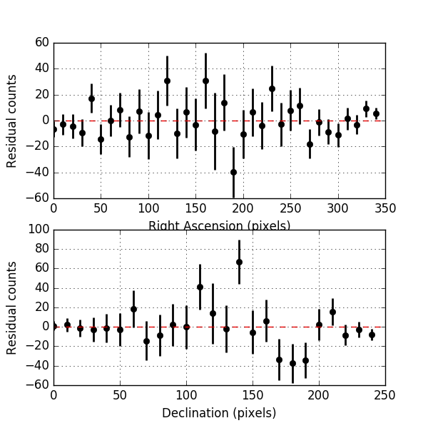
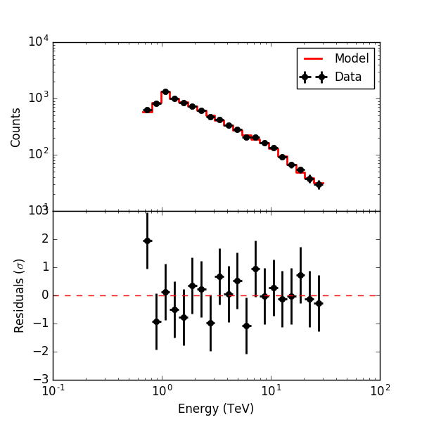
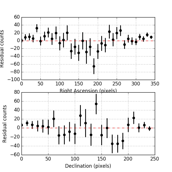
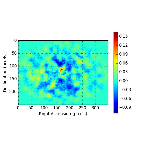
Below the residual spectrum, residual profiles in Right Ascension and Declination, and a residual map for 20 energy bins. Overall the residuals look now reasonable.
 |
 |
 |
#3
Updated by Knödlseder Jürgen about 6 years ago
- File crab_stacked20_resspec_iter1.png added
- File crab_stacked20_resprof_iter1.png added
- File crab_stacked20_resmap_iter1.png added
The background model used in ctbkgmodel was determined by fitting all observations, including the source regions. Consequently, in the ctlike fit the normalisation of the background model is reduced, as can be see in the log file, shown below for the 20 energy bins fit. In this case the background model was reduced by about 7%, the index is compatible with zero. However the shape of the background model, and the relative weighting between the backgrounds of the different observations, is preserved in a stacked analysis, introducing some bias.
2018-11-07T10:30:09: === GCTAModelCubeBackground ===
2018-11-07T10:30:09:  Name ......................: BackgroundModel
2018-11-07T10:30:09:  Instruments ...............: CTA, HESS, MAGIC, VERITAS
2018-11-07T10:30:09:  Instrument scale factors ..: unity
2018-11-07T10:30:09:  Observation identifiers ...: all
2018-11-07T10:30:09:  Model type ................: "PowerLaw" * "Constant"
2018-11-07T10:30:09:  Number of parameters ......: 4
2018-11-07T10:30:09:  Number of spectral par's ..: 3
2018-11-07T10:30:09:   Prefactor ................: 0.92688008398116 +/- 0.0138008183074852 [0.01,100] ph/cm2/s/MeV (free,scale=1,gradient)
2018-11-07T10:30:09:   Index ....................: 0.0113778958948462 +/- 0.0144446074027589 [-5,5]  (free,scale=1,gradient)
2018-11-07T10:30:09:   PivotEnergy ..............: 1000000 MeV (fixed,scale=1000000,gradient)
2018-11-07T10:30:09:  Number of temporal par's ..: 1
2018-11-07T10:30:09:   Normalization ............: 1 (relative value) (fixed,scale=1,gradient)
To understand the boas I therefore used the fit results of the unbinned analysis to generate an alternative background cube. Fitting this model to the data gives the following result. The background normalisation is now basically one. The Crab prefactor goes up by 0.15e-17, the spectral index is basically not affected. Hence the stacked analysis will somewhat underestimate the source fluxes, as expected.
2018-11-07T11:19:47: === GOptimizerLM ===
2018-11-07T11:19:47:  Optimized function value ..: 44648.462
2018-11-07T11:19:47:  Absolute precision ........: 0.005
2018-11-07T11:19:47:  Acceptable value decrease .: 2
2018-11-07T11:19:47:  Optimization status .......: converged
2018-11-07T11:19:47:  Number of parameters ......: 10
2018-11-07T11:19:47:  Number of free parameters .: 6
2018-11-07T11:19:47:  Number of iterations ......: 3
2018-11-07T11:19:47:  Lambda ....................: 1e-06
2018-11-07T11:19:47:  Maximum log likelihood ....: -44648.462
2018-11-07T11:19:47:  Observed events  (Nobs) ...: 8461.000
2018-11-07T11:19:47:  Predicted events (Npred) ..: 8455.000 (Nobs - Npred = 5.99964775683293)
2018-11-07T11:19:47: === GModels ===
2018-11-07T11:19:47:  Number of models ..........: 2
2018-11-07T11:19:47:  Number of parameters ......: 10
2018-11-07T11:19:47: === GModelSky ===
2018-11-07T11:19:47:  Name ......................: Crab
2018-11-07T11:19:47:  Instruments ...............: all
2018-11-07T11:19:47:  Test Statistic ............: 1845.6796865592
2018-11-07T11:19:47:  Instrument scale factors ..: unity
2018-11-07T11:19:47:  Observation identifiers ...: all
2018-11-07T11:19:47:  Model type ................: PointSource
2018-11-07T11:19:47:  Model components ..........: "PointSource" * "PowerLaw" * "Constant"
2018-11-07T11:19:47:  Number of parameters ......: 6
2018-11-07T11:19:47:  Number of spatial par's ...: 2
2018-11-07T11:19:47:   RA .......................: 83.6209669517135 +/- 0.00252919459519199 deg (free,scale=1)
2018-11-07T11:19:47:   DEC ......................: 22.0248642601462 +/- 0.00233953943144988 deg (free,scale=1)
2018-11-07T11:19:47:  Number of spectral par's ..: 3
2018-11-07T11:19:47:   Prefactor ................: 5.23287376743654e-17 +/- 3.38933067177766e-18 [1e-25,infty[ ph/cm2/s/MeV (free,scale=1e-17,gradient)
2018-11-07T11:19:47:   Index ....................: -2.75931417445264 +/- 0.0757563212467188 [10,-10]  (free,scale=-2,gradient)
2018-11-07T11:19:47:   PivotEnergy ..............: 1000000 MeV (fixed,scale=1000000,gradient)
2018-11-07T11:19:47:  Number of temporal par's ..: 1
2018-11-07T11:19:47:   Normalization ............: 1 (relative value) (fixed,scale=1,gradient)
2018-11-07T11:19:47: === GCTAModelCubeBackground ===
2018-11-07T11:19:47:  Name ......................: BackgroundModel
2018-11-07T11:19:47:  Instruments ...............: CTA, HESS, MAGIC, VERITAS
2018-11-07T11:19:47:  Instrument scale factors ..: unity
2018-11-07T11:19:47:  Observation identifiers ...: all
2018-11-07T11:19:47:  Model type ................: "PowerLaw" * "Constant"
2018-11-07T11:19:47:  Number of parameters ......: 4
2018-11-07T11:19:47:  Number of spectral par's ..: 3
2018-11-07T11:19:47:   Prefactor ................: 0.999715699285799 +/- 0.0148947550844672 [0.01,100] ph/cm2/s/MeV (free,scale=1,gradient)
2018-11-07T11:19:47:   Index ....................: 0.00566705715270537 +/- 0.014450942963835 [-5,5]  (free,scale=1,gradient)
2018-11-07T11:19:47:   PivotEnergy ..............: 1000000 MeV (fixed,scale=1000000,gradient)
2018-11-07T11:19:47:  Number of temporal par's ..: 1
2018-11-07T11:19:47:   Normalization ............: 1 (relative value) (fixed,scale=1,gradient)
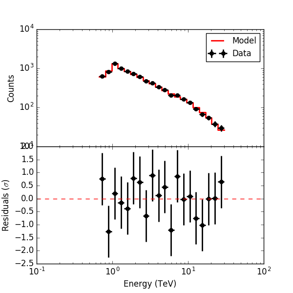
Below the residuals for the corresponding analysis. They look a bit better than the residuals before, the impact is however not dramatic.
 |
 |
 |
#4
Updated by Knödlseder Jürgen about 6 years ago
- % Done changed from 20 to 30
I also checked the results obtained with a joint binned analysis. For this purpose I created for each observation a counts cube using the usepnt=yes option. Each cube had 250 x 250 spatial bins with a bin size of 0.02 deg. 20 energy bins were used. Below the results for unbinned, stacked and joint binned analysis.
| Method | logL | TS | RA | DEC | Prefactor | Index | CPU |
| Unbinned | 98199.437 | 2025.108 | 83.623 +/- 0.002 | 22.025 +/- 0.002 | 4.892e-17 +/- 2.678e-18 | 2.702 +/- 0.066 | 48.7 |
| Stacked | 44664.118 | 1714.607 | 83.621 +/- 0.003 | 22.025 +/- 0.002 | 5.088e-17 +/- 3.361e-18 | 2.759 +/- 0.077 | 39.5 |
| Binned | 50908.047 | 1785.304 | 83.621 +/- 0.003 | 22.027 +/- 0.002 | 4.728e-17 +/- 3.006e-18 | 2.662 +/- 0.074 | 475.7 |
#5
Updated by Knödlseder Jürgen about 6 years ago
Here a comparison for 50 energy bins.
Now results between unbinned and joint binned are very close. The prefactor differs by -1.7%, the index by -1%. Statistical errors on the prefactor and index are 5.7% and 2.6%, respectively.
Differences between unbinned and stacked are +7.8% in the prefactor and +3.4% in the index.
| Method | logL | TS | RA | DEC | Prefactor | Index | CPU |
| Unbinned | 98199.437 | 2025.108 | 83.623 +/- 0.002 | 22.025 +/- 0.002 | 4.892e-17 +/- 2.678e-18 | 2.702 +/- 0.066 | 48.7 |
| Stacked | 56043.857 | 1854.033 | 83.621 +/- 0.003 | 22.024 +/- 0.002 | 5.273e-17 +/- 3.137e-18 | 2.793 +/- 0.073 | 84.6 |
| Binned | 63003.006 | 1938.315 | 83.621 +/- 0.003 | 22.027 +/- 0.002 | 4.811e-17 +/- 2.756e-18 | 2.675 +/- 0.069 | 771.6 |
#6
Updated by Knödlseder Jürgen about 6 years ago
I varied some parameters of the response cube computation to see whether they impact the fit results.
| Method | logL | TS | RA | DEC | Prefactor | Index | CPU |
| Unbinned | 98199.437 | 2025.108 | 83.623 +/- 0.002 | 22.025 +/- 0.002 | 4.892e-17 +/- 2.678e-18 | 2.702 +/- 0.066 | 48.7 |
| Stacked | 44664.118 | 1714.607 | 83.621 +/- 0.003 | 22.025 +/- 0.002 | 5.088e-17 +/- 3.361e-18 | 2.759 +/- 0.077 | 39.5 |
| amax=1.0 | 44663.161 | 1716.523 | 83.621 +/- 0.003 | 22.024 +/- 0.003 | 5.082e-17 +/- 3.350e-18 | 2.760 +/- 0.077 | 21.4 |
| amax=1.0, abins=1000 | 44663.174 | 1716.497 | 83.621 +/- 0.003 | 22.024 +/- 0.003 | 5.085e-17 +/- 3.354e-18 | 2.760 +/- 0.077 | 25.3 |
| psf=cnt(1) | 44664.104 | 1714.636 | 83.621 +/- 0.003 | 22.025 +/- 0.002 | 5.088e-17 +/- 3.361e-18 | 2.759 +/- 0.077 | 28.2 |
| psf ebins=100 | 44663.967 | 1714.910 | 83.621 +/- 0.003 | 22.025 +/- 0.002 | 5.095e-17 +/- 3.364e-18 | 2.760 +/- 0.077 | 15.9 |
| exp ebins=30 | 44662.694 | 1717.457 | 83.621 +/- 0.003 | 22.025 +/- 0.002 | 5.210e-17 +/- 3.436e-18 | 2.778 +/- 0.077 | 19.4 |
| exp ebins=40 | 44662.283 | 1718.278 | 83.621 +/- 0.003 | 22.025 +/- 0.002 | 4.775e-17 +/- 3.128e-18 | 2.705 +/- 0.076 | 23.0 |
| exp ebins=50 | 44661.381 | 1720.082 | 83.621 +/- 0.003 | 22.025 +/- 0.002 | 4.904e-17 +/- 3.214e-18 | 2.727 +/- 0.077 | 20.0 |
| exp ebins=60 | 44661.005 | 1720.835 | 83.621 +/- 0.003 | 22.025 +/- 0.002 | 5.036e-17 +/- 3.305e-18 | 2.749 +/- 0.077 | 20.1 |
| exp ebins=70 | 44663.801 | 1715.242 | 83.621 +/- 0.003 | 22.025 +/- 0.002 | 4.807e-17 +/- 3.160e-18 | 2.711 +/- 0.077 | 24.2 |
| exp ebins=80 | 44662.283 | 1718.278 | 83.621 +/- 0.003 | 22.025 +/- 0.002 | 4.775e-17 +/- 3.128e-18 | 2.705 +/- 0.076 | 24.1 |
| exp ebins=90 | 44661.365 | 1720.115 | 83.621 +/- 0.003 | 22.025 +/- 0.002 | 4.907e-17 +/- 3.217e-18 | 2.728 +/- 0.077 | 19.7 |
| exp ebins=100 | 44662.283 | 1718.278 | 83.621 +/- 0.003 | 22.025 +/- 0.002 | 4.775e-17 +/- 3.128e-18 | 2.705 +/- 0.076 | 23.3 |
| exp ebins=110 | 44662.284 | 1718.277 | 83.621 +/- 0.003 | 22.025 +/- 0.002 | 4.775e-17 +/- 3.128e-18 | 2.705 +/- 0.076 | 24.1 |
| exp ebins=120 | 44662.283 | 1718.278 | 83.621 +/- 0.003 | 22.025 +/- 0.002 | 4.775e-17 +/- 3.128e-18 | 2.705 +/- 0.076 | 24.7 |
| exp ebins=130 | 44662.283 | 1718.279 | 83.621 +/- 0.003 | 22.025 +/- 0.002 | 4.775e-17 +/- 3.128e-18 | 2.705 +/- 0.076 | 23.9 |
| exp full=300(2) | 44662.283 | 1718.278 | 83.621 +/- 0.003 | 22.025 +/- 0.002 | 4.775e-17 +/- 3.128e-18 | 2.705 +/- 0.076 | 23.5 |
(1) psf=cnt means that the counts cube definition was used to define the PSF cube
(2) exposure cube computed over full 100 GeV - 100 TeV energy range with 300 energy bins
It turns out that the precise number of energy bins used for the exposure cube computation has an impact on the results, and with a finer energy binning the stacked analysis results get close to the unbinned analysis result. The H.E.S.S. effective area is provided for 96 bins within 100 GeV and 100 TeV, meaning that there are 24 bins per decade. The 0.67-30 TeV range used in this analysis is 1.7 decades, covering about 40 energy bins of the effective area IRF. Sampling the exposure cube with 40 bins provides indeed a result that is very close to the unbinned analysis, however increasing the number of energy bins worsens the result. Only from 100 energy bins on the result seems to converge towards a value close to the unbinned analysis result, meaning that at about a factor of 3 oversampling of the IRF is appropriate for the stacked analysis.
Since for energy dispersion a wider energy range is needed in the exposure cube, I also tried computing 300 energy bins over the full 100 GeV - 100 TeV energy range, which corresponds to about a factor of 3 oversampling in true energy. Also this works nicely, as the table shows.
#7
Updated by Knödlseder Jürgen about 6 years ago
I now changed the Crab analysis script, computing the exposure cube, the PSF cube and the energy dispersion cube for the full energy range of 100 GeV - 100 TeV with 300 energy bins. Below the result comparison for unbinned, stacked and binned analysis. The binned analysis was redone using the new ctbin tool that now also produces multiple counts cubes. As before, 20 energy bins were used for the counts cube(s). Results are now reasonably close.
| Method | logL | TS | RA | DEC | Prefactor | Index | CPU |
| Unbinned | 98199.437 | 2025.108 | 83.623 +/- 0.002 | 22.025 +/- 0.002 | 4.892e-17 +/- 2.678e-18 | 2.702 +/- 0.066 | 48.7 |
| Stacked | 44662.282 | 1718.280 | 83.621 +/- 0.003 | 22.025 +/- 0.002 | 4.778e-17 +/- 3.130e-18 | 2.706 +/- 0.076 | 38.7 |
| Binned | 50908.055 | 1785.288 | 83.621 +/- 0.003 | 22.027 +/- 0.002 | 4.729e-17 +/- 3.007e-18 | 2.663 +/- 0.074 | 306.0 |
#8
Updated by Knödlseder Jürgen about 6 years ago
Here now the same results for energy dispersion enabled.
| Method | logL | TS | RA | DEC | Prefactor | Index | CPU |
| Unbinned | 98196.591 | 2030.800 | 83.622 +/- 0.003 | 22.024 +/- 0.002 | 4.148e-17 +/- 2.005e-18 | 2.734 +/- 0.070 | 116.4 |
| Stacked | 44683.345 | 1676.155 | 83.620 +/- 0.003 | 22.025 +/- 0.003 | 5.859e-17 +/- 3.557e-18 | 3.587 +/- 0.126 | 3570.4 |
| Binned | 50905.009 | 1791.382 | 83.620 +/- 0.003 | 22.026 +/- 0.003 | 4.130e-17 +/- 2.271e-18 | 2.721 +/- 0.078 | 5698 |
The stacked results look really bad. Something is going wrong with the energy dispersion there.
#9
Updated by Knödlseder Jürgen about 6 years ago
- Status changed from New to In Progress
- % Done changed from 30 to 40
I inspected the GCTAEdispCube::operator() interface and revised it according to the GCTAEdisp::operator() interface. Now the GCTAEdispCube::operator() takes the reconstructed and true energy in form of GEnergy objects, followed by the true sky direction.
I also corrected the GCTAEdispCube::set() method which performed some incorrect exposure weighting. This has been fixed. I added unit tests to make sure that the energy dispersion cube when integrated over reconstructed energy for a given set of true energies is unity. The tests are performed for the GCTAEdispCube::set() and GCTAEdispCube::fill() methods, hence we can be sure that the methods actually work.
#10
Updated by Knödlseder Jürgen about 6 years ago
I now investigated different parameters for the ctedispcube tool.
| Method | logL | TS | RA | DEC | Prefactor | Index | CPU |
| Unbinned | 98196.591 | 2030.800 | 83.622 +/- 0.003 | 22.024 +/- 0.002 | 4.148e-17 +/- 2.005e-18 | 2.734 +/- 0.070 | 116.4 |
| max=2.0, bins=100 | 44683.345 | 1676.155 | 83.620 +/- 0.003 | 22.025 +/- 0.003 | 5.859e-17 +/- 3.557e-18 | 3.587 +/- 0.126 | 3570.4 |
| max=5.0, bins=300 | 44659.671 | 1723.503 | 83.620 +/- 0.003 | 22.024 +/- 0.003 | 5.596e-17 +/- 3.620e-18 | 2.999 +/- 0.094 | 3177.9 |
| max=5.0, bins=500 | 44659.491 | 1723.862 | 83.620 +/- 0.003 | 22.025 +/- 0.005 | 5.633e-17 +/- 3.650e-18 | 3.007 +/- 0.094 | 3287.1 |
Increasing the number of energy bins does not resolve the issue.
#11
Updated by Knödlseder Jürgen about 6 years ago
I checked whether the cutting of response values where the true energy falls outside the valid reconstructed energy interval has an impact on the analysis results. Below the results. All runs were done using max=5.0 and bins=300.
| Method | logL | TS | RA | DEC | Prefactor | Index | CPU |
| Unbinned | 98196.591 | 2030.800 | 83.622 +/- 0.003 | 22.024 +/- 0.002 | 4.148e-17 +/- 2.005e-18 | 2.734 +/- 0.070 | 116.4 |
| Cutting | 44659.671 | 1723.503 | 83.620 +/- 0.003 | 22.024 +/- 0.003 | 5.596e-17 +/- 3.620e-18 | 2.999 +/- 0.094 | 3177.9 |
| No cut of Edisp | 44659.806 | 1723.233 | 83.620 +/- 0.003 | 22.025 +/- 0.003 | 5.498e-17 +/- 3.535e-18 | 2.984 +/- 0.093 | 3732.4 |
| No cut of Aeff and Edisp | 44657.592 | 1727.660 | 83.621 +/- 0.003 | 22.024 +/- 0.003 | 3.854e-17 +/- 2.167e-18 | 2.689 +/- 0.080 | 2245.3 |
| No cut of Aeff, PSF and Edisp | 44656.980 | 1728.884 | 83.621 +/- 0.003 | 22.024 +/- 0.003 | 3.891e-17 +/- 2.184e-18 | 2.698 +/- 0.080 | 882.0 |
#12
Updated by Knödlseder Jürgen about 6 years ago
It seems best to disable the true energy cut in all response cube computation tools. Here again the summary for unbinned, stacked and binned analysis using energy dispersion.
| Method | logL | TS | RA | DEC | Prefactor | Index | CPU |
| Unbinned | 98196.591 | 2030.800 | 83.622 +/- 0.003 | 22.024 +/- 0.002 | 4.148e-17 +/- 2.005e-18 | 2.734 +/- 0.070 | 116.4 |
| Stacked | 44656.980 | 1728.884 | 83.621 +/- 0.003 | 22.024 +/- 0.003 | 3.891e-17 +/- 2.184e-18 | 2.698 +/- 0.080 | 882.0 |
| Binned | 50905.009 | 1791.382 | 83.620 +/- 0.003 | 22.026 +/- 0.003 | 4.130e-17 +/- 2.271e-18 | 2.721 +/- 0.078 | 5698 |
#13
Updated by Knödlseder Jürgen about 6 years ago
- File image.png added
- File screenshot_2_1541779166_image.png added
I now also redid the analysis with the new stacked response cubes without cuts. For some reason the results differs from the former result Not clear what happened.
| Edisp | logL | TS | RA | DEC | Prefactor | Index | CPU |
| No (former result) | 44662.282 | 1718.280 | 83.621 +/- 0.003 | 22.025 +/- 0.002 | 4.778e-17 +/- 3.130e-18 | 2.706 +/- 0.076 | 38.7 |
| No | 44658.674 | 1725.497 | 83.621 +/- 0.003 | 22.025 +/- 0.002 | 4.555e-17 +/- 2.946e-18 | 2.662 +/- 0.075 | 44.2 |
| Yes | 44656.985 | 1728.874 | 83.621 +/- 0.003 | 22.024 +/- 0.003 | 3.890e-17 +/- 2.183e-18 | 2.697 +/- 0.080 | 1746.3 |
I therefore progressively put back the true energy cuts to check what’s going on. Without energy dispersion, cutting in true energy should be more realistic since it avoids spill-over in energy.
| Cutting | logL | TS | RA | DEC | Prefactor | Index | CPU |
| No | 44658.674 | 1725.497 | 83.621 +/- 0.003 | 22.025 +/- 0.002 | 4.555e-17 +/- 2.946e-18 | 2.662 +/- 0.075 | 44.2 |
| Aeff cut | 44662.270 | 1718.304 | 83.621 +/- 0.003 | 22.025 +/- 0.002 | 4.793e-17 +/- 3.136e-18 | 2.708 +/- 0.076 | 39.1 |
| PSF cut | 44658.753 | 1725.339 | 83.621 +/- 0.003 | 22.025 +/- 0.002 | 4.544e-17 +/- 2.942e-18 | 2.660 +/- 0.075 | 39.2 |
| Aeff & PSF cut | 44662.066 | 1718.713 | 83.621 +/- 0.003 | 22.025 +/- 0.002 | 4.785e-17 +/- 3.132e-18 | 2.707 +/- 0.076 | 39.9 |
| Aeff & PSF cut (former result) | 44662.282 | 1718.280 | 83.621 +/- 0.003 | 22.025 +/- 0.002 | 4.778e-17 +/- 3.130e-18 | 2.706 +/- 0.076 | 38.7 |
The impact of the PSF cut is negligible, which is understandable since the exact weight of the PSF between the various observations should not be relevant. The important cut is the Aeff cut. Cutting on both gives similar results to the Aeff cut alone, which is expected since the PSF cut is negligible.
Still, we don’t get exactly the same results are before, which may be due a different energy binning used for the PSF.
So to summarise:- spill-over leads to a bias in the prefactor of -4.8% and in the index of -1.7% without energy dispersion
- spill-over leads to a bias in the prefactor of -6.2% and in the index of -1.3% with energy dispersion (reference = unbinned)
#14
Updated by Knödlseder Jürgen about 6 years ago
- File deleted (
screenshot_2_1541779166_image.png)
#15
Updated by Knödlseder Jürgen about 6 years ago
- File deleted (
image.png)
#16
Updated by Knödlseder Jürgen about 6 years ago
I now also explored different number of reconstructed energy bins, since at the very beginning of this thread this also led to different spectral results. For comparison I also repeat the unbinned results.
| Bins | Edisp | Clipping | logL | TS | Prefactor | Index | CPU |
| - | No | - | 98199.437 | 2025.108 | 4.892e-17 +/- 2.678e-18 | 2.702 +/- 0.066 | 48.7 |
| 20 | No | No | 44658.674 | 1725.497 | 4.555e-17 +/- 2.946e-18 | 2.662 +/- 0.075 | 44.2 |
| 40 | No | No | 54061.014 | 1872.168 | 4.650e-17 +/- 2.731e-18 | 2.675 +/- 0.071 | 86.8 |
| 60 | No | No | 57605.204 | 1880.635 | 4.753e-17 +/- 2.764e-18 | 2.696 +/- 0.071 | 136.8 |
| Bins | Edisp | Clipping | logL | TS | Prefactor | Index | CPU |
| - | No | - | 98199.437 | 2025.108 | 4.892e-17 +/- 2.678e-18 | 2.702 +/- 0.066 | 48.7 |
| 20 | No | Yes | 44662.066 | 1718.713 | 4.785e-17 +/- 3.132e-18 | 2.707 +/- 0.076 | 39.9 |
| 40 | No | Yes | 54063.421 | 1867.353 | 5.251e-17 +/- 3.132e-18 | 2.785 +/- 0.073 | 83.8 |
| 60 | No | Yes | 57613.687 | 1863.669 | 5.348e-17 +/- 3.174e-18 | 2.806 +/- 0.073 | 151.3 |
| Bins | Edisp | Clipping | logL | TS | Prefactor | Index | CPU |
| - | Yes | - | 98196.591 | 2030.800 | 4.148e-17 +/- 2.005e-18 | 2.734 +/- 0.070 | 116.4 |
| 20 | Yes | No | 44656.985 | 1728.874 | 3.890e-17 +/- 2.183e-18 | 2.697 +/- 0.080 | 1746.3 |
| 40 | Yes | No | 54059.809 | 1874.578 | 3.932e-17 +/- 2.032e-18 | 2.670 +/- 0.076 | 3278.0 |
| 60 | Yes | No | 57602.555 | 1885.932 | 3.994e-17 +/- 2.040e-18 | 2.718 +/- 0.076 | 4327.9 |
| Bins | Edisp | Clipping | logL | TS | Prefactor | Index | CPU |
| - | Yes | - | 98196.591 | 2030.800 | 4.148e-17 +/- 2.005e-18 | 2.734 +/- 0.070 | 116.4 |
| 20 | Yes | Yes | 44659.671 | 1723.503 | 5.596e-17 +/- 3.620e-18 | 2.999 +/- 0.094 | 3177.9 |
| 40 | Yes | Yes | 54060.554 | 1873.088 | 5.833e-17 +/- 3.433e-18 | 3.041 +/- 0.090 | 6075.4 |
| 60 | Yes | Yes | 57609.798 | 1871.447 | 5.975e-17 +/- 3.498e-18 | 3.073 +/- 0.090 | 4520.3 |
#17
Updated by Knödlseder Jürgen about 6 years ago
- File spill-over_40bins_amax03_anumbins200_noclip.png added
- File spill-over_40bins_amax03_anumbins200_clip.png added
- File spill-over_40bins_amax07_anumbins300_clip.png added
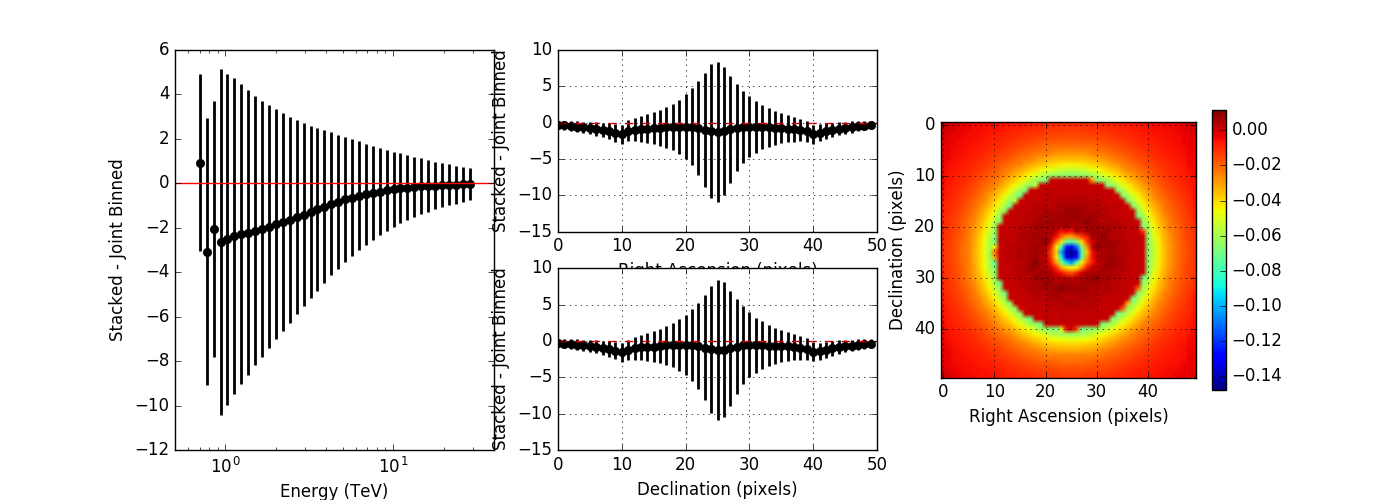
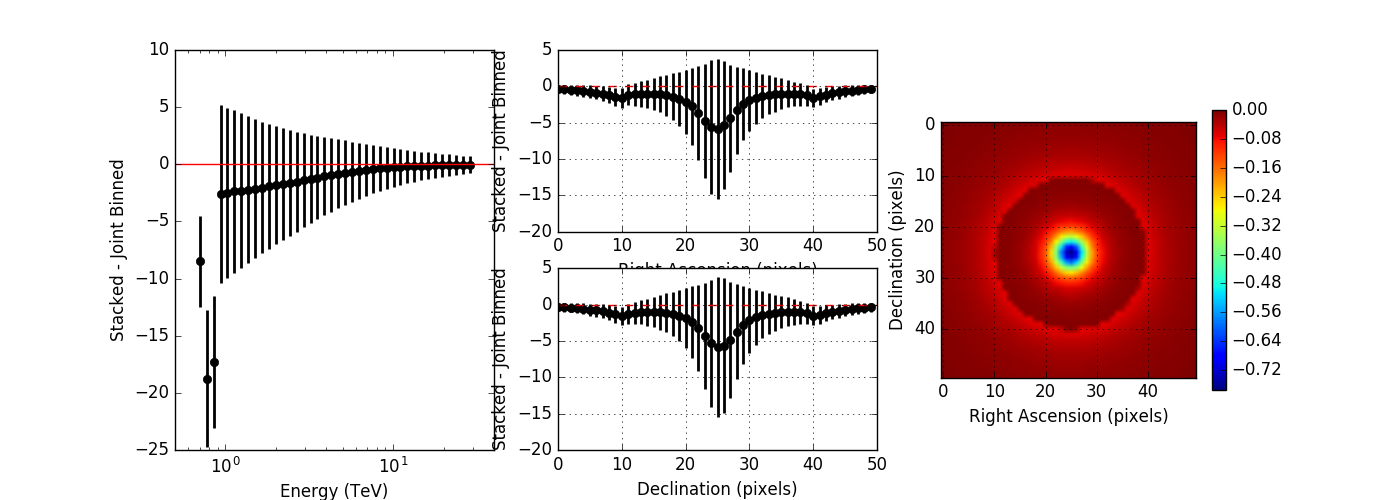
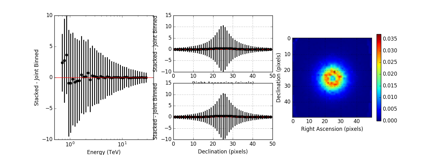
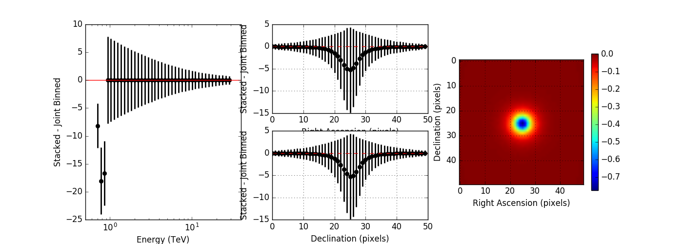
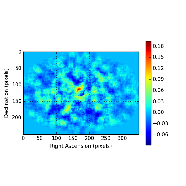
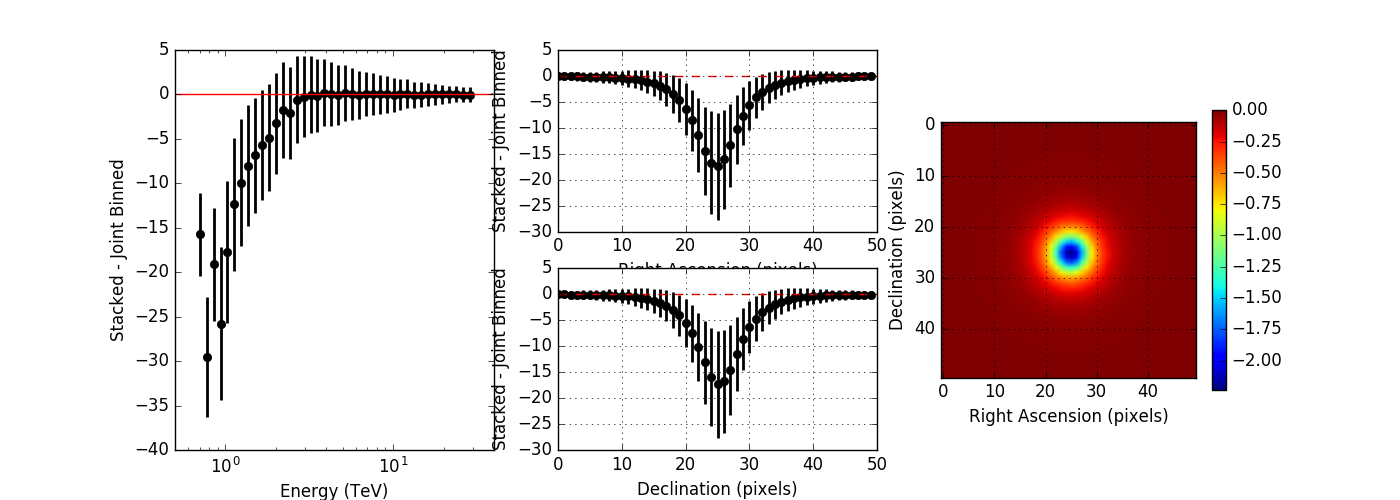
I compared the model counts computed using an unbinned observation to the model counts computed using a stacked observation to study the effect of the spill over. The figures below show the residual of the stacked model minus the joint binned model. Left panels show the spectral residuals, central panels the spatial residual profiles in Right Ascension and Declination, and the right panels a residual map integrated over all energies. The top panels show the residuals without clipping, the bottom panel show the residuals with clipping. Obviously, clipping leads to a strong residual at low energies, near the threshold of the observations. Not clipping the stacked response is therefore strongly preferred.


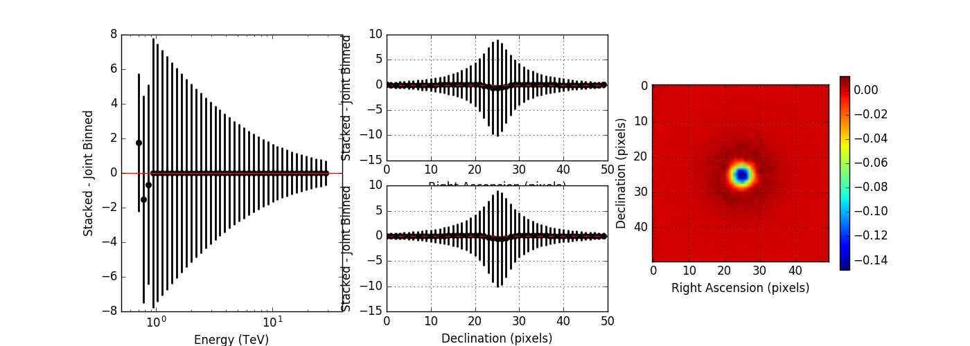
The non-clipped residuals show an energy dependent trend, where only at high energies, the computation is identical. This indicates that the stacked PSF cube may not fully comprise the H.E.S.S. PSF. I therefore increased the maximum PSF angle from 0.2 degrees to 0.7 degrees which covers the angles provided in the H.E.S.S. IRF. I also set the number of angular bins to 300, which gives an ovsersampling by a factor of 2 of the PSF. The image below shows, obtained without clipping, that this solves the residual trend.

#18
Updated by Knödlseder Jürgen about 6 years ago
- File spill-over_40bins_amax07_anumbins300_noclip_edisp.png added
#19
Updated by Knödlseder Jürgen about 6 years ago
- File deleted (
spill-over_40bins_amax07_anumbins300_noclip_edisp.png)
#20
Updated by Knödlseder Jürgen about 6 years ago
- File deleted (
spill-over_40bins_amax07_anumbins300_clip.png)
#21
Updated by Knödlseder Jürgen about 6 years ago
#22
Updated by Knödlseder Jürgen about 6 years ago
- File spill-over_40bins_amax07_anumbins300_noclip_edisp.png added
- File spill-over_40bins_amax07_anumbins300_clip.png added
- File spill-over_40bins_amax07_anumbins300_clip_edisp.png added
- % Done changed from 40 to 80
Here the plots without and with energy dispersion for no clipping:

And now with clipping enabled:

From these plots it is obvious that the stacked response should not be clipped. I therefore changed the code.
#23
Updated by Knödlseder Jürgen about 6 years ago
- File show_spill_over.py added
For the record, attached the script to generate the spill over plot: show_spill_over.py
#24
Updated by Knödlseder Jürgen about 6 years ago
Here now the final stacked results as function of the number of energy bins, in comparison to the unbinned results. The results converge for 40-50 energy bins, corresponding to about 20-25 energy bins per decade.
| Bins | Edisp | logL | TS | Prefactor | Index | CPU |
| - | No | 98199.437 | 2025.108 | 4.892e-17 +/- 2.678e-18 | 2.702 +/- 0.066 | 48.7 |
| 20 | No | 44658.100 | 1726.645 | 4.546e-17 +/- 2.934e-18 | 2.663 +/- 0.075 | 35.3 |
| 40 | No | 54060.675 | 1872.846 | 4.637e-17 +/- 2.718e-18 | 2.675 +/- 0.071 | 69.2 |
| 50 | No | 56036.742 | 1868.261 | 4.692e-17 +/- 2.735e-18 | 2.689 +/- 0.071 | 103.3 |
| 60 | No | 57604.533 | 1881.977 | 4.740e-17 +/- 2.750e-18 | 2.695 +/- 0.071 | 130.9 |
| 80 | No | 60446.160 | 1872.688 | 4.641e-17 +/- 2.718e-18 | 2.676 +/- 0.071 | 212.8 |
| Bins | Edisp | logL | TS | Prefactor | Index | CPU |
| - | Yes | 98196.591 | 2030.800 | 4.148e-17 +/- 2.005e-18 | 2.734 +/- 0.070 | 116.4 |
| 20 | Yes | 44656.563 | 1729.718 | 3.883e-17 +/- 2.174e-18 | 2.698 +/- 0.080 | 1423.6 |
| 40 | Yes | 54059.739 | 1874.717 | 3.918e-17 +/- 2.022e-18 | 2.698 +/- 0.076 | 2737.0 |
| 50 | Yes | 56034.364 | 1873.019 | 3.951e-17 +/- 2.022e-18 | 2.712 +/- 0.075 | 3402.5 |
| 60 | Yes | 57602.116 | 1886.812 | 3.985e-17 +/- 2.031e-18 | 2.718 +/- 0.075 | 3920.5 |
| 80 | Yes | 61382.504 | 1874.959 | 3.922e-17 +/- 2.021e-18 | 2.670 +/- 0.076 | 5192.3 |
#25
Updated by Knödlseder Jürgen about 6 years ago
- File crab_sed_ptsrc_plaw_gauss_grad_hess_binned40_edisp.png added
- File crab_sed_ptsrc_plaw_gauss_grad_hess_binned40.png added
- File crab_sed_ptsrc_plaw_gauss_grad_hess_edisp.png added
- File crab_sed_ptsrc_plaw_gauss_grad_hess_stacked40_edisp.png added
- File crab_sed_ptsrc_plaw_gauss_grad_hess_stacked40.png added
- File crab_sed_ptsrc_plaw_gauss_grad_hess.png added
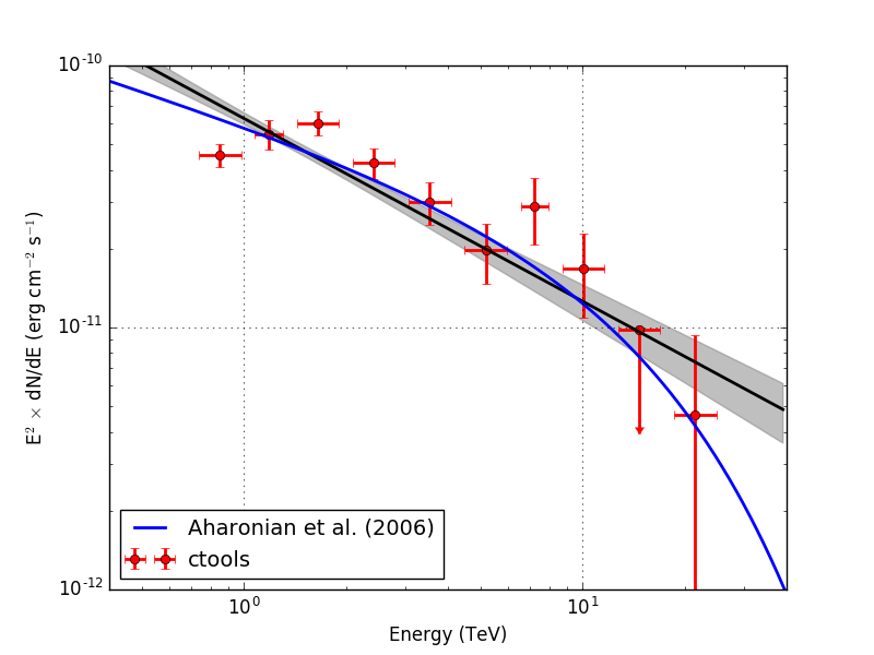
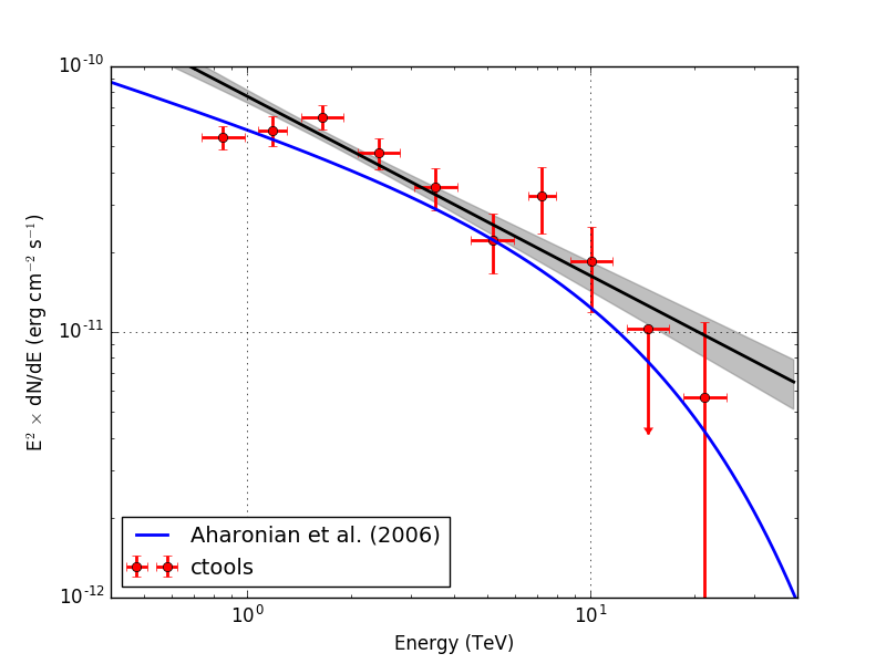
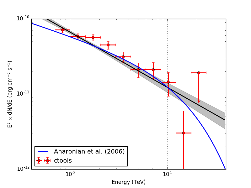
Below the spectra obtained using an unbinned, joint binned and stacked analysis. Note that the energy bins for the binned and stacked analysis are not aligned with the bin boundaries of the counts cube, which explains the gaps in the spectrum. The joined binned and stacked analysis results are very similar.
| Method | No energy dispersion | Energy dispersion |
| Unbinned | 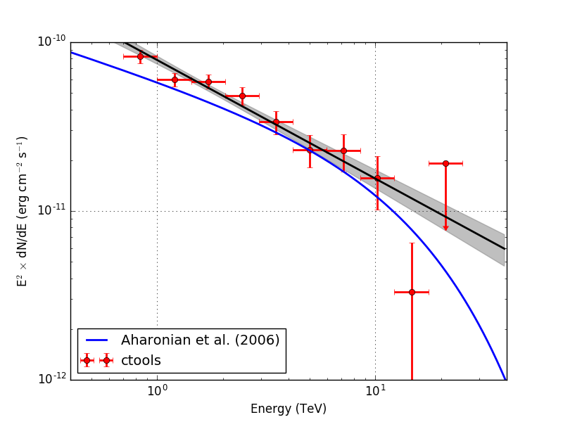 |
 |
| Binned |  |
 |
| Stacked | 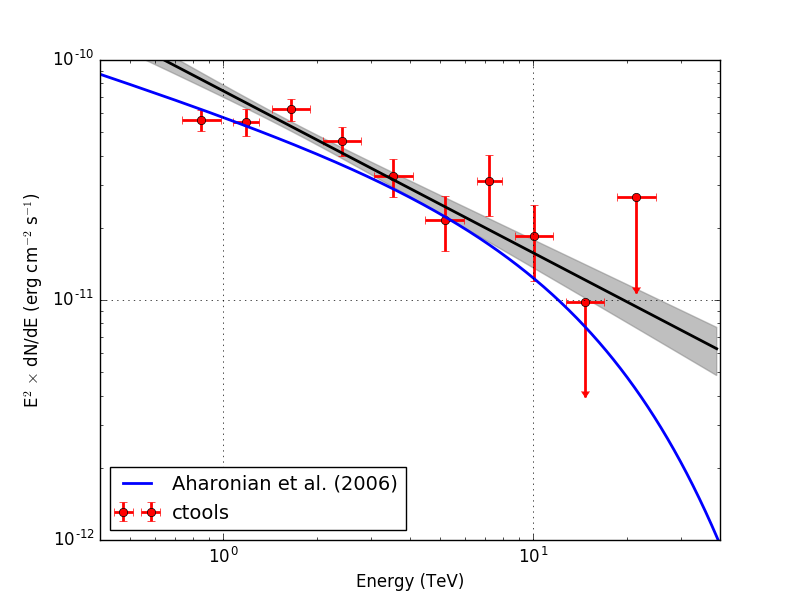 |
 |
#26
Updated by Knödlseder Jürgen about 6 years ago
#27
Updated by Knödlseder Jürgen about 6 years ago
- File deleted (
crab_sed_ptsrc_plaw_gauss_grad_hess_binned40.png)
#28
Updated by Knödlseder Jürgen about 6 years ago
- File deleted (
crab_sed_ptsrc_plaw_gauss_grad_hess_binned40_edisp.png)
#29
Updated by Knödlseder Jürgen about 6 years ago
#30
Updated by Knödlseder Jürgen about 6 years ago
I also checked the RX J1713.7-3946 observation. Below the results for unbinned and stacked analysis (40 energy bins). Energy dispersion was not applied. The stacked analysis provides a lower prefactor than the unbinned analysis, as expected due to the overestimation of the background model. The background prefactor for the stacked analysis was 0.963.
| Analysis | logL | TS | Prefactor | Index | Cutoff (TeV) | Bkg. prefactor |
| Unbinned | 537778.100 | 741.007 | 2.025e-17 +/- 1.983e-18 | 1.925 +/- 0.118 | 5.569 +/- 2.057 | - |
| Stacked | 212467.591 | 688.935 | 1.776e-17 +/- 1.483e-18 | 1.931 +/- 0.108 | 7.092 +/- 2.612 | 0.963 +/- 0.005 |
#31
Updated by Knödlseder Jürgen about 6 years ago
- Status changed from In Progress to Closed
- % Done changed from 80 to 100
I consider that the stacked analysis is now checked.