Action #1304: Improve fitting convergence behavior for ellipse models - GammaLib - CTA IRAP Project Gateway

Action #1304

Improve fitting convergence behavior for ellipse models

Added by Knödlseder Jürgen almost 10 years ago. Updated over 9 years ago.

Status:

Closed

Start date:

07/28/2014

Priority:

Normal

Due date:

Assigned To:

Knödlseder Jürgen

% Done:

100%

Category:

Estimated time:

0.00 hour

Target version:

00-09-00

Duration:

Description

Fitting of ellipse models takes many iterations, indicating bad convergence behavior, likely related to numerical noise in the gradient computations. This should be improved.

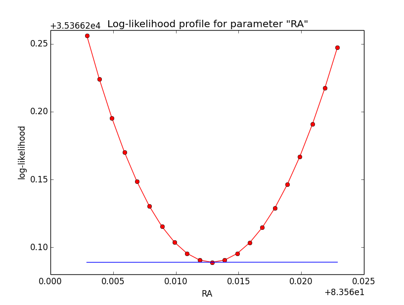
likeprf_ra_1e3.png (37.1 KB) Knödlseder Jürgen, 10/29/2014 12:25 AM

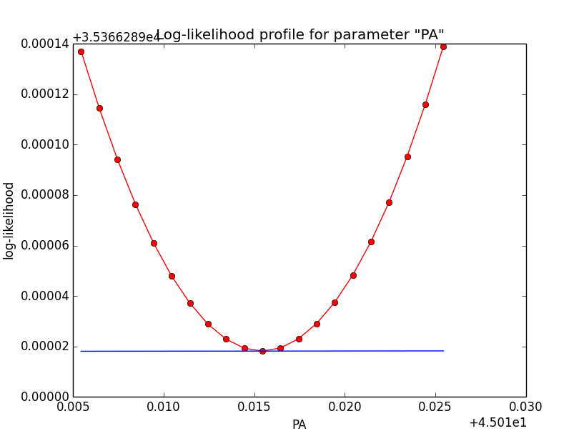
likeprf_dec_1e3.png (39.3 KB) Knödlseder Jürgen, 10/29/2014 12:25 AM

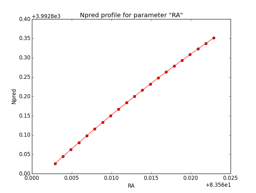
likeprf_pa_1e3.png (46.3 KB) Knödlseder Jürgen, 10/29/2014 12:25 AM

npredprf_ra_1e3.png (35 KB) Knödlseder Jürgen, 10/29/2014 12:25 AM

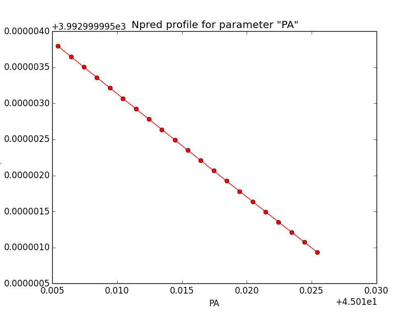
npredprf_dec_1e3.png (35.5 KB) Knödlseder Jürgen, 10/29/2014 12:25 AM

npredprf_pa_1e3.png (43.7 KB) Knödlseder Jürgen, 10/29/2014 12:25 AM

likeprf_major_1e3.png (43.3 KB) Knödlseder Jürgen, 10/29/2014 01:45 AM

likeprf_minor_1e3.png (37.7 KB) Knödlseder Jürgen, 10/29/2014 01:45 AM

npredprf_major_1e3.png (34 KB) Knödlseder Jürgen, 10/29/2014 01:45 AM

npredprf_minor_1e3.png (36.5 KB) Knödlseder Jürgen, 10/29/2014 01:45 AM

Recurrence

No recurrence.

Related issues

History

#1 Updated by Knödlseder Jürgen almost 10 years ago

Here the trigonometric ellipse equations (with PA counted counterclockwise from North, where X=RA and Y=Dec):

X(phi) = X0 + a cos(phi) * sin(PA) - b sin(phi) * cos(PA)
Y(phi) = Y0 + a cos(phi) * cos(PA) + b sin(phi) * sin(PA)

which compares to the equations of a circle (PA=0, a=b) at the same centre:

X(phi) = X0 + r cos(phi)
Y(phi) = Y0 + r sin(phi)

Maybe a solution could be to determine the two arcs of a circle with the same centre at a given distance r from the ellipse centre, and to determine the intersection of these arcs with another circle. This basically will give new limits for the two arcs, which can then be used for integration on a circle.

#2 Updated by Knödlseder Jürgen over 9 years ago

After updating the code so that integration is only restricted to the elliptical region, the following benchmark has been obtained for the elliptical model (see #1299 for previous analysis):

Implementation	Unbinned	Binned	Stacked
Prevision	151.9 sec (32, 35349.603, 83.626, 21.998, 44.725, 0.497, 1.994)	14291.3 sec (46, 19946.631, 83.627, 22.011, 44.980, 0.482, 1.940, 5.351e-16, -2.487)	- not finished -
New	167.141 (14, 35363.715, 83.570, 21.958, 44.793, 0.473, 1.997, 5.4291e-16, -2.482)	2144.2 sec (6, 19943.976, 83.571, 21.956, 44.908, 0.474, 1.988, 5.332e-16, -2.473)	6782.1 sec (16, 19944.430, 83.571, 21.957, 44.93, 2.006, 0.467, 5.312e-16, -2.444

The reference values are:

Parameter	Value
RA	83.6331
DEC	22.0145
PA	45.0
MajorRadius	2.0
MinorRadius	0.5
Prefactor	5.7e-7
Index	-2.48

Notes:

the precision of the optimizer has been set to 1e-3; before it was 1e-6 and this led to many iterations for the binned analysis jumping from the negative slope to the positive slope and back, indicating some noise in the gradient computation that prevents quick convergence
for unbinned analysis there were 7 stalls before convergence was reached
it has been checked that inverting semimajor and semiminor axis and increasing the position angle by 90 to get the same ellipse does also work; this means that the code is not sensitive to the condition semimajor > semiminor, it also works for semimajor < semiminor

#3 Updated by Knödlseder Jürgen over 9 years ago

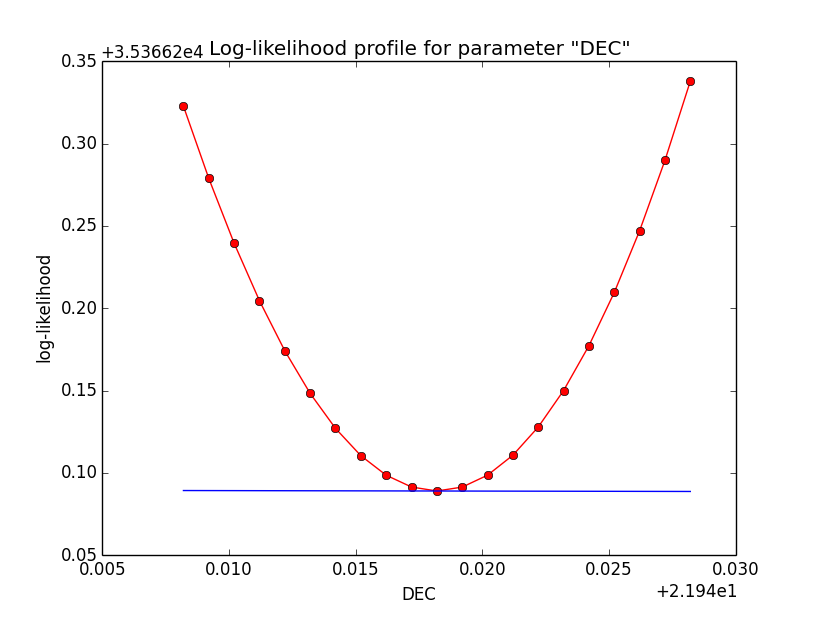
File likeprf_ra_1e3.png added
File likeprf_dec_1e3.png added
File likeprf_pa_1e3.png added
File npredprf_ra_1e3.png added
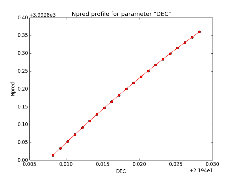
File npredprf_dec_1e3.png added
File npredprf_pa_1e3.png added

Below the likelihood profiles (first row) and the Npred profiles (second row) for the parameters Right Ascension (RA), Declination (DEC) and Position angle (PA) after restricting the computation to an ellipse. Everything is nice and smooth now.

#4 Updated by Knödlseder Jürgen over 9 years ago

Status changed from New to In Progress
Assigned To set to Knödlseder Jürgen
Target version set to 00-09-00
% Done changed from 0 to 50

#5 Updated by Knödlseder Jürgen over 9 years ago

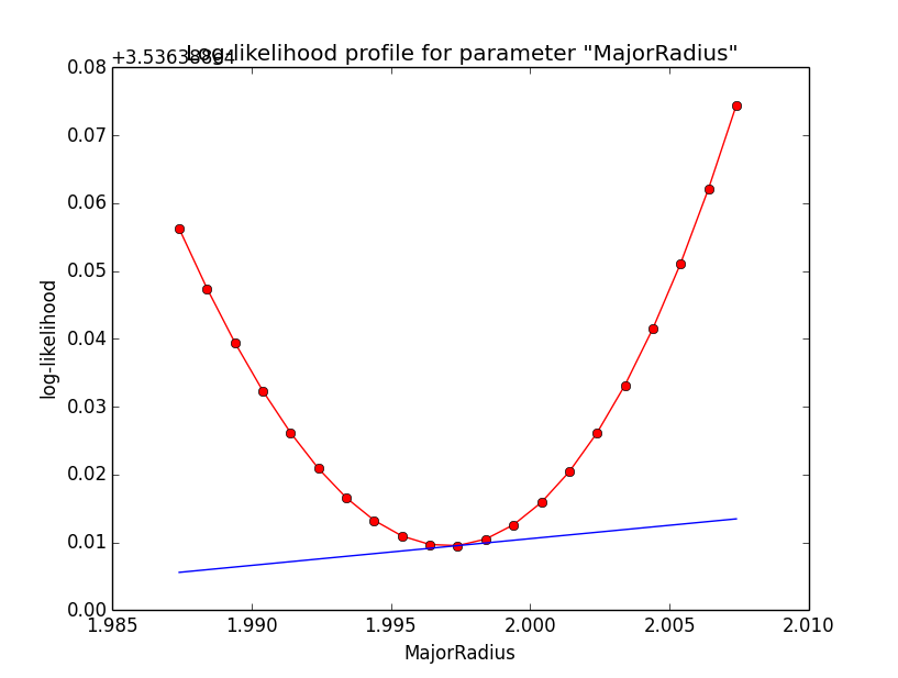
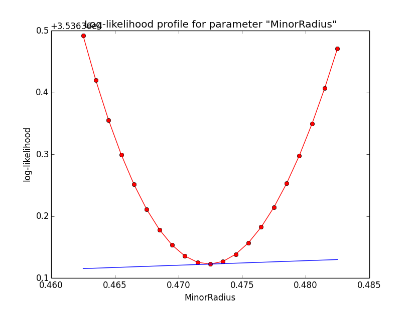
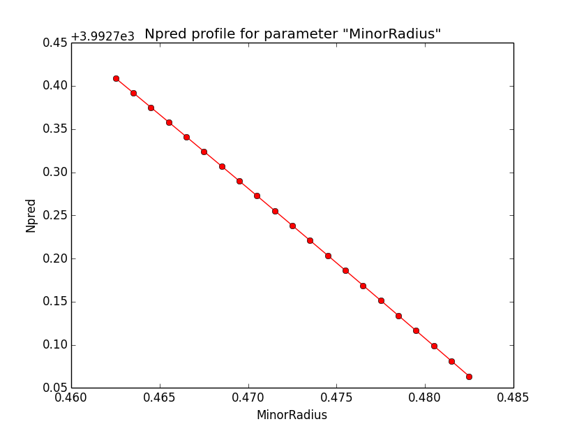
File likeprf_major_1e3.png added
File likeprf_minor_1e3.png added
File npredprf_major_1e3.png added
File npredprf_minor_1e3.png added

And here the profiles for the SemiMajor and SemiMinor axes.

#6 Updated by Knödlseder Jürgen over 9 years ago

Status changed from In Progress to Closed
% Done changed from 50 to 100
Remaining (hours) set to 0.0

This is now solved (see benchmark in #1291). Close the issue now.

#7 Updated by Knödlseder Jürgen over 9 years ago

Status changed from Closed to In Progress
% Done changed from 100 to 90
Estimated time set to 0.00

I re-open this as there is still an issue with the stacked analysis. Below the actual benchmark results (timed on kepler):

Model	Unbinned	Binned	Stacked
Ellipse	156.9 sec (5, 35363.713, 83.569, 21.956, 44.789, 1.998, 0.472, 5.430e-16, -2.482)	5754.1 sec (6, 19943.973, 83.572, 21.956, 44.909, 1.988, 0.474, 5.331e-16, -2.473)	13337.0 sec (14 of which 7 stalled, 19945.148, 83.528, 21.922, 44.768, 1.986, 0.479, 5.337e-16, -2.441)

There are 7 stalls for the stacked analysis, and the code takes quite some time. Not clear why this now appears as I had a working code before. I also cross-check the code, the stacked integration code is identical to the binned code, just the response computation part is of course different.

To see whether I can adjust the iter_rho and iter_phi parameters, here the results from the IRF computation:

iter_rho	iter_phi	Events	CPU time
5	5	-5.335 events (-0.6%)	42.578 sec
4	6	-32.265 events (-3.8%)	40.967 sec
5	6	0.471 events (0.1%)	70.303 sec
6	4	-40.612 events (-4.8%)	52.828 sec
6	5	-1.251 events (-0.1%)	79.460 sec

#8 Updated by Knödlseder Jürgen over 9 years ago

I tried fitting using iter_rho=5 and iter_phi=6 and this still gives stalls:

>Iteration   0: -logL=19949.209, Lambda=1.0e-03
>Iteration   1: -logL=19947.792, Lambda=1.0e-03, delta=1.417, max(|grad|)=-45.320641 [MajorRadius:3]
>Iteration   2: -logL=19945.231, Lambda=1.0e-04, delta=2.561, max(|grad|)=-30.478977 [MajorRadius:3]
>Iteration   3: -logL=19944.779, Lambda=1.0e-05, delta=0.452, max(|grad|)=-23.095176 [RA:0]
 Iteration   4: -logL=19944.779, Lambda=1.0e-06, delta=-0.081, max(|grad|)=25.939015 [RA:0] (stalled)
 Iteration   5: -logL=19944.779, Lambda=1.0e-05, delta=-0.081, max(|grad|)=25.948140 [RA:0] (stalled)
 Iteration   6: -logL=19944.779, Lambda=1.0e-04, delta=-0.080, max(|grad|)=26.037961 [RA:0] (stalled)

#9 Updated by Knödlseder Jürgen over 9 years ago

Also with iter_rho=6 and iter_phi=5 things are not better:

>Iteration   0: -logL=19950.777, Lambda=1.0e-03
>Iteration   1: -logL=19948.821, Lambda=1.0e-03, delta=1.956, max(|grad|)=-58.339344 [MajorRadius:3]
>Iteration   2: -logL=19945.009, Lambda=1.0e-04, delta=3.812, max(|grad|)=-24.732729 [MajorRadius:3]
>Iteration   3: -logL=19944.221, Lambda=1.0e-05, delta=0.788, max(|grad|)=-4.299682 [RA:0]
>Iteration   4: -logL=19944.203, Lambda=1.0e-06, delta=0.018, max(|grad|)=3.396798 [RA:0]
 Iteration   5: -logL=19944.203, Lambda=1.0e-07, delta=-0.002, max(|grad|)=-5.865259 [DEC:1] (stalled)
 Iteration   6: -logL=19944.203, Lambda=1.0e-06, delta=-0.002, max(|grad|)=-5.864910 [DEC:1] (stalled)
 Iteration   7: -logL=19944.203, Lambda=1.0e-05, delta=-0.002, max(|grad|)=-5.861274 [DEC:1] (stalled)
 Iteration   8: -logL=19944.203, Lambda=1.0e-04, delta=-0.002, max(|grad|)=-5.827261 [DEC:1] (stalled)
 Iteration   9: -logL=19944.203, Lambda=1.0e-03, delta=-0.002, max(|grad|)=-5.513205 [DEC:1] (stalled)
 Iteration  10: -logL=19944.203, Lambda=1.0e-02, delta=-0.001, max(|grad|)=-3.878288 [DEC:1] (stalled)
>Iteration  11: -logL=19944.195, Lambda=1.0e-01, delta=0.007, max(|grad|)=-3.275571 [MinorRadius:4]

#10 Updated by Knödlseder Jürgen over 9 years ago

I implemented a quadatric binning in GCTAMeanPsf that allows using of a faster linear interpolation scheme for the Psf. This led however only to a marginal speed increase:

Scheme	Events	CPU time
Non-linear interpolation	-5.335 events (-0.6%)	42.578 sec
Linear interpolation	-5.367 events (-0.6%)	35.123 sec	Linear interpolation, additional transition point	-5.340 events (-0.6%)	43.670 sec

I also made a test with an additional transition point

double transition_point = delta_max - rho_obs;
if (transition_point > rho_min && transition_point < rho_max) {
    bounds.push_back(transition_point);
}

I did this as I still do not understand why the fitting worked without stalls at some time in the past. The transition point is the one for radial models, and I’m not sure why it should have some relevance for an elliptical model, but I give it a try.

#11 Updated by Knödlseder Jürgen over 9 years ago

Now here the fitting results using linear interpolation (on Mac OS X for the times):

>Iteration   0: -logL=19950.488, Lambda=1.0e-03
>Iteration   1: -logL=19947.943, Lambda=1.0e-03, delta=2.544, max(|grad|)=-47.192988 [MajorRadius:3]
>Iteration   2: -logL=19945.535, Lambda=1.0e-04, delta=2.409, max(|grad|)=-17.940678 [MajorRadius:3]
>Iteration   3: -logL=19945.329, Lambda=1.0e-05, delta=0.206, max(|grad|)=-11.948178 [MinorRadius:4]
>Iteration   4: -logL=19945.287, Lambda=1.0e-06, delta=0.042, max(|grad|)=11.002294 [RA:0]
>Iteration   5: -logL=19945.243, Lambda=1.0e-07, delta=0.043, max(|grad|)=-11.110490 [MinorRadius:4]
>Iteration   6: -logL=19945.157, Lambda=1.0e-08, delta=0.086, max(|grad|)=-5.432131 [DEC:1]
>Iteration   7: -logL=19945.144, Lambda=1.0e-09, delta=0.013, max(|grad|)=-3.332762 [MinorRadius:4]
>Iteration   8: -logL=19945.143, Lambda=1.0e-10, delta=0.001, max(|grad|)=-5.401481 [DEC:1]
=== GOptimizerLM ===
 Optimized function value ..: 19945.143
 Absolute precision ........: 0.005
 Optimization status .......: converged
 Number of parameters ......: 14
 Number of free parameters .: 10
 Number of iterations ......: 8
 Lambda ....................: 1e-11
=== GModels ===
 Number of models ..........: 2
 Number of parameters ......: 14
=== GModelSky ===
 Name ......................: Gaussian Crab
 Instruments ...............: all
 Instrument scale factors ..: unity
 Observation identifiers ...: all
 Model type ................: ExtendedSource
 Model components ..........: "EllipticalDisk" * "PowerLaw" * "Constant" 
 Number of parameters ......: 9
 Number of spatial par's ...: 5
  RA .......................: 83.5271 +/- 0.0239564 [-360,360] deg (free,scale=1)
  DEC ......................: 21.9197 +/- 0.0223213 [-90,90] deg (free,scale=1)
  PA .......................: 44.7764 +/- 0.513999 [-360,360] deg (free,scale=1)
  MajorRadius ..............: 1.98321 +/- 0.0463111 [0.001,10] deg (free,scale=1)
  MinorRadius ..............: 0.47961 +/- 0.0125513 [0.001,10] deg (free,scale=1)
 Number of spectral par's ..: 3
  Prefactor ................: 5.33731e-16 +/- 3.44191e-17 [1e-23,1e-13] ph/cm2/s/MeV (free,scale=1e-16,gradient)
  Index ....................: -2.44175 +/- 0.039501 [-0,-5]  (free,scale=-1,gradient)
  PivotEnergy ..............: 300000 [10000,1e+09] MeV (fixed,scale=1e+06,gradient)
 Number of temporal par's ..: 1
  Constant .................: 1 (relative value) (fixed,scale=1,gradient)
=== GCTAModelRadialAcceptance ===
 Name ......................: Background
 Instruments ...............: CTA
 Instrument scale factors ..: unity
 Observation identifiers ...: all
 Model type ................: "Gaussian" * "PowerLaw" * "Constant" 
 Number of parameters ......: 5
 Number of radial par's ....: 1
  Sigma ....................: 2.97689 +/- 0.0800541 [0.01,10] deg2 (free,scale=1,gradient)
 Number of spectral par's ..: 3
  Prefactor ................: 6.28973e-05 +/- 2.42314e-06 [0,0.001] ph/cm2/s/MeV (free,scale=1e-06,gradient)
  Index ....................: -1.85424 +/- 0.0194663 [-0,-5]  (free,scale=-1,gradient)
  PivotEnergy ..............: 1e+06 [10000,1e+09] MeV (fixed,scale=1e+06,gradient)
 Number of temporal par's ..: 1
  Constant .................: 1 (relative value) (fixed,scale=1,gradient)
Elapsed time ..............: 3488.071 sec

Interestingly, the change in the interpolation method changed the convergence behavior. This illustrates once more that the fitting is quite sensitive of details in the computation.

And here with the additional transition point:

>Iteration   0: -logL=19950.515, Lambda=1.0e-03
>Iteration   1: -logL=19947.237, Lambda=1.0e-03, delta=3.278, max(|grad|)=41.066397 [MinorRadius:4]
>Iteration   2: -logL=19944.937, Lambda=1.0e-04, delta=2.300, max(|grad|)=18.750487 [MinorRadius:4]
>Iteration   3: -logL=19944.510, Lambda=1.0e-05, delta=0.427, max(|grad|)=9.184525 [DEC:1]
>Iteration   4: -logL=19944.489, Lambda=1.0e-06, delta=0.022, max(|grad|)=5.877595 [RA:0]
>Iteration   5: -logL=19944.475, Lambda=1.0e-07, delta=0.014, max(|grad|)=2.597646 [RA:0]
>Iteration   6: -logL=19944.471, Lambda=1.0e-08, delta=0.004, max(|grad|)=-3.707069 [MinorRadius:4]
=== GOptimizerLM ===
 Optimized function value ..: 19944.471
 Absolute precision ........: 0.005
 Optimization status .......: converged
 Number of parameters ......: 14
 Number of free parameters .: 10
 Number of iterations ......: 6
 Lambda ....................: 1e-09
=== GModels ===
 Number of models ..........: 2
 Number of parameters ......: 14
=== GModelSky ===
 Name ......................: Gaussian Crab
 Instruments ...............: all
 Instrument scale factors ..: unity
 Observation identifiers ...: all
 Model type ................: ExtendedSource
 Model components ..........: "EllipticalDisk" * "PowerLaw" * "Constant" 
 Number of parameters ......: 9
 Number of spatial par's ...: 5
  RA .......................: 83.5724 +/- 0.0259483 [-360,360] deg (free,scale=1)
  DEC ......................: 21.958 +/- 0.0240572 [-90,90] deg (free,scale=1)
  PA .......................: 44.9278 +/- 0.556725 [-360,360] deg (free,scale=1)
  MajorRadius ..............: 2.0072 +/- 0.0501483 [0.001,10] deg (free,scale=1)
  MinorRadius ..............: 0.466658 +/- 0.0117936 [0.001,10] deg (free,scale=1)
 Number of spectral par's ..: 3
  Prefactor ................: 5.31439e-16 +/- 3.42817e-17 [1e-23,1e-13] ph/cm2/s/MeV (free,scale=1e-16,gradient)
  Index ....................: -2.44439 +/- 0.0394781 [-0,-5]  (free,scale=-1,gradient)
  PivotEnergy ..............: 300000 [10000,1e+09] MeV (fixed,scale=1e+06,gradient)
 Number of temporal par's ..: 1
  Constant .................: 1 (relative value) (fixed,scale=1,gradient)
=== GCTAModelRadialAcceptance ===
 Name ......................: Background
 Instruments ...............: CTA
 Instrument scale factors ..: unity
 Observation identifiers ...: all
 Model type ................: "Gaussian" * "PowerLaw" * "Constant" 
 Number of parameters ......: 5
 Number of radial par's ....: 1
  Sigma ....................: 2.96759 +/- 0.0791897 [0.01,10] deg2 (free,scale=1,gradient)
 Number of spectral par's ..: 3
  Prefactor ................: 6.32395e-05 +/- 2.42331e-06 [0,0.001] ph/cm2/s/MeV (free,scale=1e-06,gradient)
  Index ....................: -1.85288 +/- 0.0194006 [-0,-5]  (free,scale=-1,gradient)
  PivotEnergy ..............: 1e+06 [10000,1e+09] MeV (fixed,scale=1e+06,gradient)
 Number of temporal par's ..: 1
  Constant .................: 1 (relative value) (fixed,scale=1,gradient)
 Elapsed time ..............: 2885.634 sec

This has a more steady decrease of the -logL and also converges a little faster, leading to a net improvement in the end. I’ll keep that one for the moment. I’ll close the issue now and created a new one (#1355) to follow-up on this in the future.

#12 Updated by Knödlseder Jürgen over 9 years ago

Status changed from In Progress to Closed
% Done changed from 90 to 100

Also available in: Atom PDF

	Related to GammaLib - Bug #1299: Fitting problems with radial disk model	Closed	07/25/2014
	Related to GammaLib - Change request #1355: Try doing the elliptical CTA response computation in a Ps...	New	10/31/2014

GammaLib

Issues

Tags