Bug #1299

Fitting problems with radial disk model
| Status: | Closed | Start date: | 07/25/2014 | |
|---|---|---|---|---|
| Priority: | Normal | Due date: | ||
| Assigned To: |  Knödlseder Jürgen Knödlseder Jürgen | % Done: | 100% | |
| Category: | - | |||
| Target version: | 00-09-00 | |||
| Duration: |
Description
While finalizing the stacked cube analysis (#1291) I encountered a problem with fitting the radial disk model. For stacked cube analysis, the fit converges badly. But even for unbinned analysis, the fit takes many iterations. Here for example a log for unbinned fitting:
>Iteration   0: -logL=34182.372, Lambda=1.0e-03
>Iteration   1: -logL=34180.081, Lambda=1.0e-03, delta=2.290, max(|grad|)=19.555723 [DEC:1]
>Iteration   2: -logL=34180.070, Lambda=1.0e-04, delta=0.011, max(|grad|)=-6.847438 [Radius:2]
>Iteration   3: -logL=34180.070, Lambda=1.0e-05, delta=0.001, max(|grad|)=2.516642 [Radius:2]
>Iteration   4: -logL=34180.070, Lambda=1.0e-06, delta=0.000, max(|grad|)=-3.717756 [Radius:2]
 Iteration   5: -logL=34180.070, Lambda=1.0e-07, delta=-0.000, max(|grad|)=3.502109 [Radius:2] (stalled)
 Iteration   6: -logL=34180.070, Lambda=1.0e-06, delta=-0.000, max(|grad|)=3.502427 [Radius:2] (stalled)
 Iteration   7: -logL=34180.070, Lambda=1.0e-05, delta=-0.000, max(|grad|)=3.501858 [Radius:2] (stalled)
 Iteration   8: -logL=34180.070, Lambda=1.0e-04, delta=-0.000, max(|grad|)=3.501880 [Radius:2] (stalled)
 Iteration   9: -logL=34180.070, Lambda=1.0e-03, delta=-0.000, max(|grad|)=3.499197 [Radius:2] (stalled)
 Iteration  10: -logL=34180.070, Lambda=1.0e-02, delta=-0.000, max(|grad|)=3.455784 [Radius:2] (stalled)
 Iteration  11: -logL=34180.070, Lambda=1.0e-01, delta=-0.000, max(|grad|)=2.826601 [Radius:2] (stalled)
 Iteration  12: -logL=34180.070, Lambda=1.0e+00, delta=-0.000, max(|grad|)=2.395730 [Radius:2] (stalled)
>Iteration  13: -logL=34180.070, Lambda=1.0e+01, delta=0.000, max(|grad|)=-3.178778 [DEC:1]
 Iteration  14: -logL=34180.070, Lambda=1.0e+00, delta=-0.000, max(|grad|)=2.706520 [DEC:1] (stalled)
 Iteration  15: -logL=34180.070, Lambda=1.0e+01, delta=-0.000, max(|grad|)=-1.960376 [RA:0] (stalled)
>Iteration  16: -logL=34180.070, Lambda=1.0e+02, delta=0.000, max(|grad|)=-1.937920 [RA:0]
=== GObservations ===
 Number of observations ....: 1
 Number of predicted events : 4038
=== GModelSky ===
 Number of spatial par's ...: 3
  RA .......................: 83.6324 +/- 0.00394119 [-360,360] deg (free,scale=1)
  DEC ......................: 22.0138 +/- 0.00327793 [-90,90] deg (free,scale=1)
  Radius ...................: 0.201159 +/- 0.00305998 [0.01,10] deg (free,scale=1)
 Number of spectral par's ..: 3
  Prefactor ................: 5.45432e-16 +/- 1.99357e-17 [1e-23,1e-13] ph/cm2/s/MeV (free,scale=1e-16,gradient)
  Index ....................: -2.45887 +/- 0.0267077 [-0,-5]  (free,scale=-1,gradient)
=== GCTAModelRadialAcceptance ===
 Number of radial par's ....: 1
  Sigma ....................: 3.05822 +/- 0.039788 [0.01,10] deg2 (free,scale=1,gradient)
 Number of spectral par's ..: 3
  Prefactor ................: 5.99601e-05 +/- 1.76021e-06 [0,0.001] ph/cm2/s/MeV (free,scale=1e-06,gradient)
  Index ....................: -1.85301 +/- 0.0164761 [-0,-5]  (free,scale=-1,gradient)
The fit stalls often (which is also the case for binned and stacked cube analysis) and takes many iterations to terminate. Note that for the above example, the numerical integration step size was set to 1e-5.
disk_unbin_scale3_DEC.png (38.7 KB)
disk_unbin_scale3_RA.png (38.7 KB)
disk_unbin_scale3_Radius.png (35 KB)
disk_unbin_scale4_DEC.png (39.6 KB)
disk_unbin_scale4_RA.png (39.6 KB)
disk_unbin_scale4_Radius.png (39.5 KB)
disk_unbin_scale5_DEC.png (53.1 KB)
disk_unbin_scale5_RA.png (50.2 KB)
disk_unbin_scale5_Radius.png (43.5 KB)
disk_unbin_Npred_DEC.png (43.7 KB)
disk_unbin_Npred_RA.png (46.7 KB)
disk_unbin_Npred_Radius.png (41.9 KB)
disk_unbin_scale5_DE_r2a2.png (42.7 KB)
disk_unbin_scale5_RA_r2a2.png (50.5 KB)
disk_unbin_scale5_Radius_r2a2.png (44.9 KB)
disk_bin_scale5_Radius_r2a2.png (46 KB)
disk_bin_scale5_RA_r2a2.png (51.5 KB)
disk_bin_scale5_DEC_r2a2.png (42.9 KB)
gauss_unbin_scale5_RA_r2a2.png (45.6 KB)
gauss_unbin_scale5_RA_r5a5.png (37.6 KB)
no-azimuth-integration.png (46.9 KB)
integration-psf.png (13.5 KB)
integration-model.png (12.4 KB)
disk_unbin-model_scale5_RA_prec5_grad0002.png (49 KB)
disk_unbin-model-switch_scale5_RA_prec5_grad0002.png (47.1 KB)
gauss_5iter.png (47.5 KB)
gauss_6iter.png (46.3 KB)
gauss_7iter.png (46.9 KB)
disk_7iter_prec5-diff.png (51 KB)
disk_6iter_prec5-diff.png (41.7 KB)
disk_5iter_prec5-diff.png (51.1 KB)
disk_psf-switch_5iter_prec5-diff.png (42.8 KB)
disk_psf-switch_8iter_prec5-diff.png (43.7 KB)


Recurrence
No recurrence.
Related issues
History
#1
 Updated by Knödlseder Jürgen over 10 years ago
- Description updated (diff)
#2
Updated by Knödlseder Jürgen over 10 years ago
- Description updated (diff)
#3
Updated by Knödlseder Jürgen over 10 years ago
- File disk_unbin_scale3_DEC.png added
- File disk_unbin_scale3_RA.png added
- File disk_unbin_scale3_Radius.png added
- File disk_unbin_scale4_DEC.png added
- File disk_unbin_scale4_RA.png added
- File disk_unbin_scale4_Radius.png added
- File disk_unbin_scale5_DEC.png added
- File disk_unbin_scale5_RA.png added
- File disk_unbin_scale5_Radius.png added
Problem description
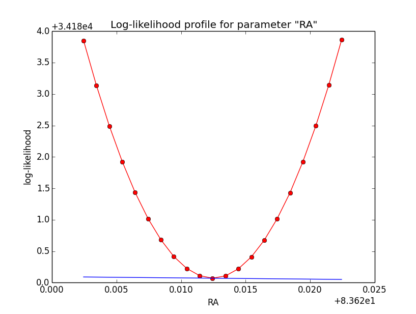
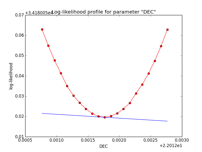
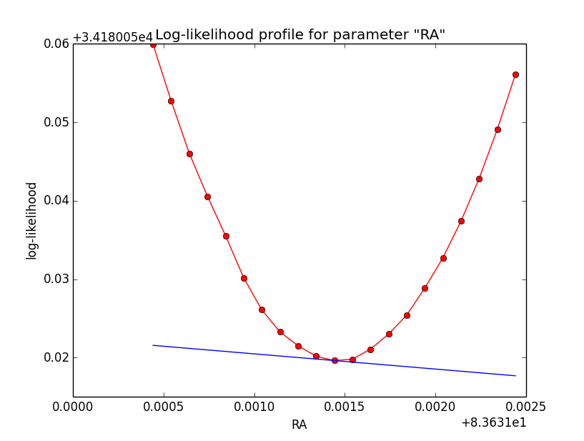
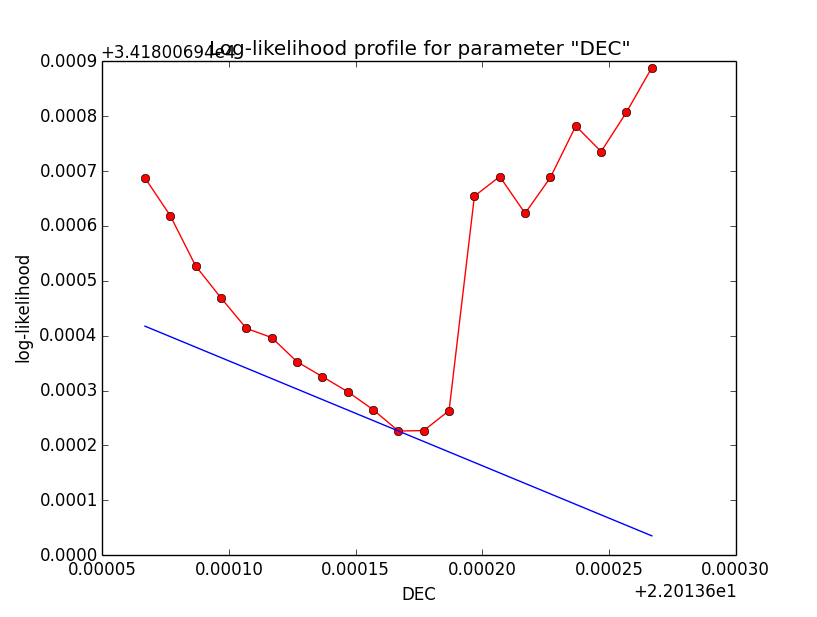
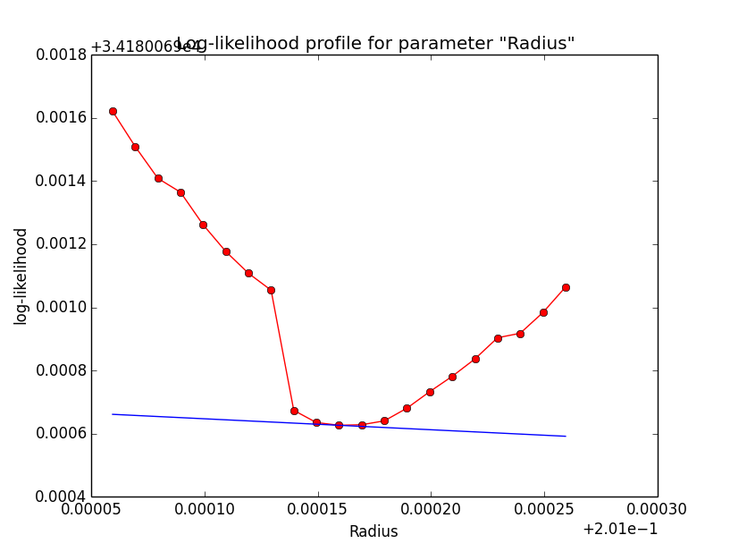
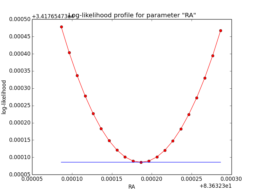
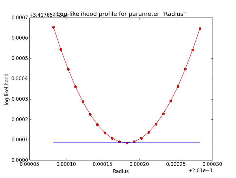
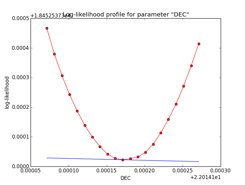
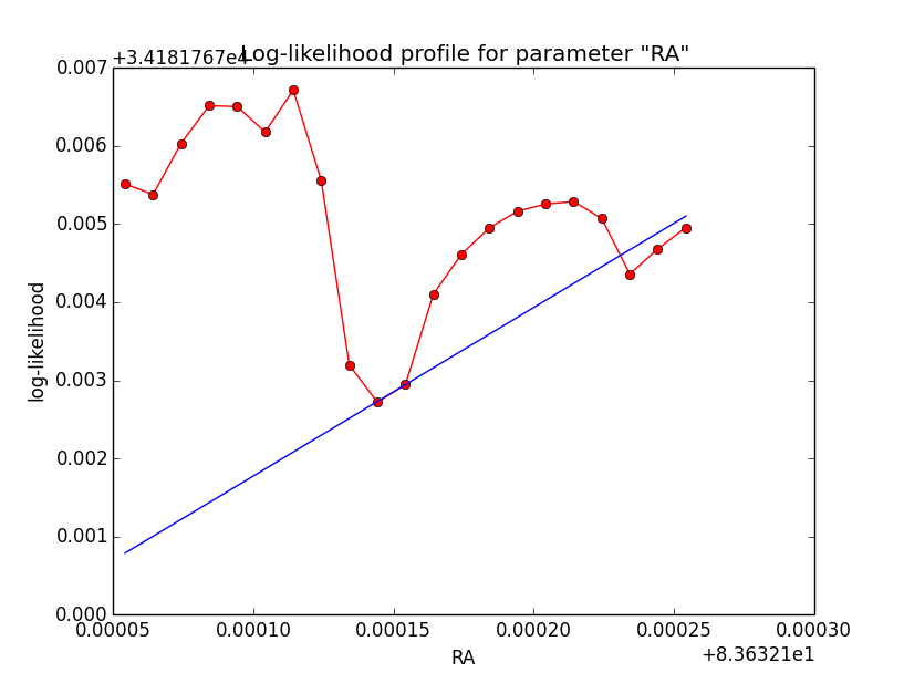
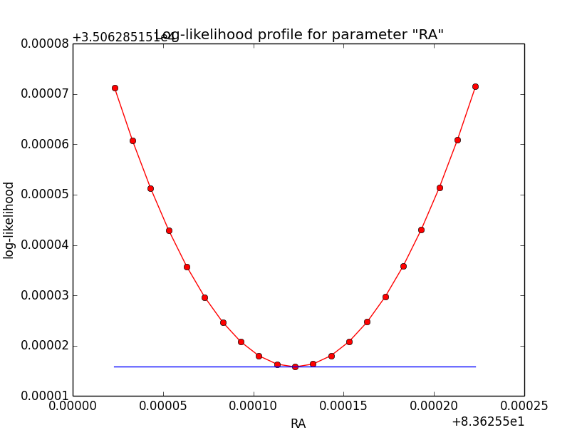
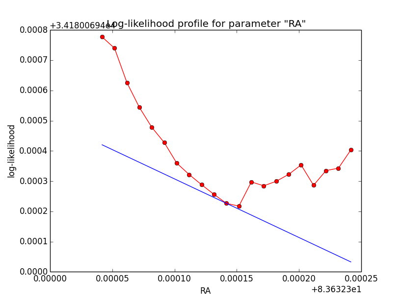
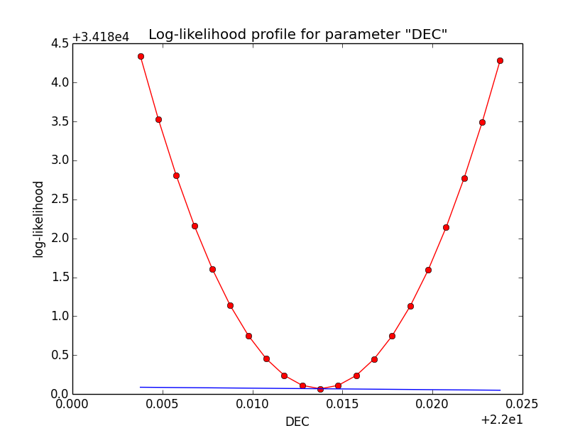
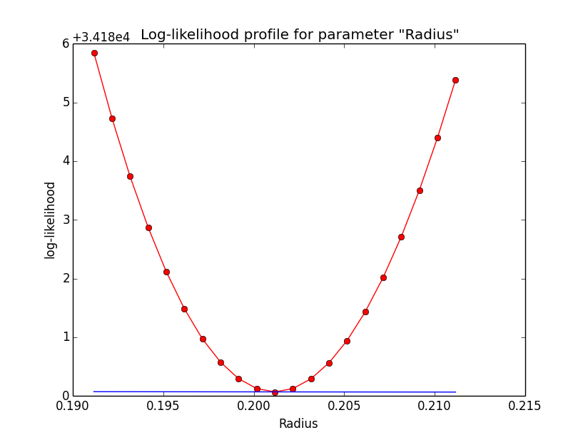
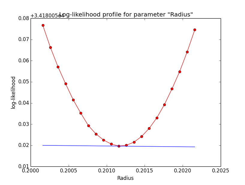
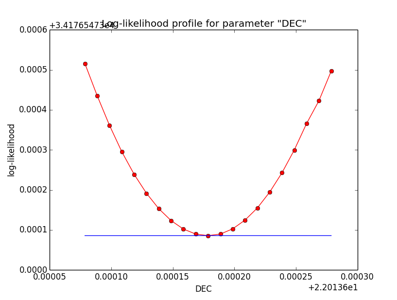
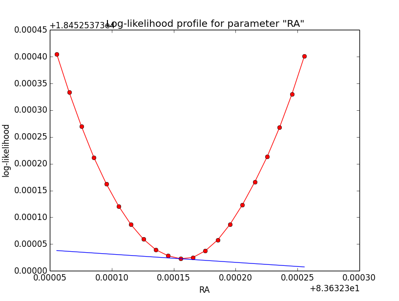
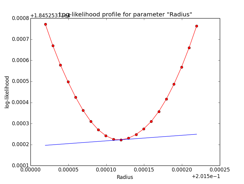
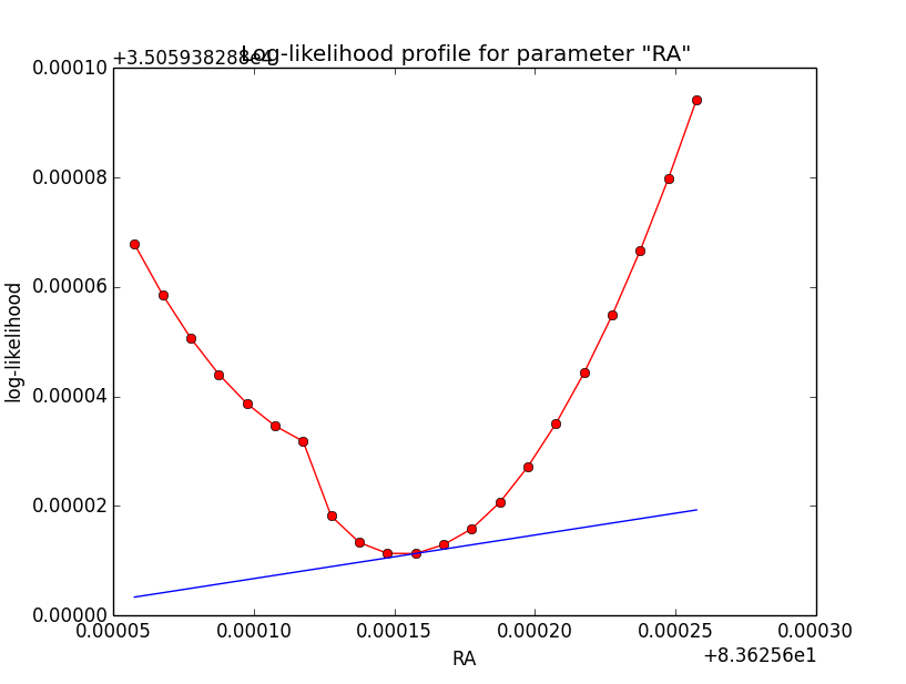
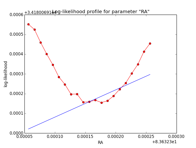
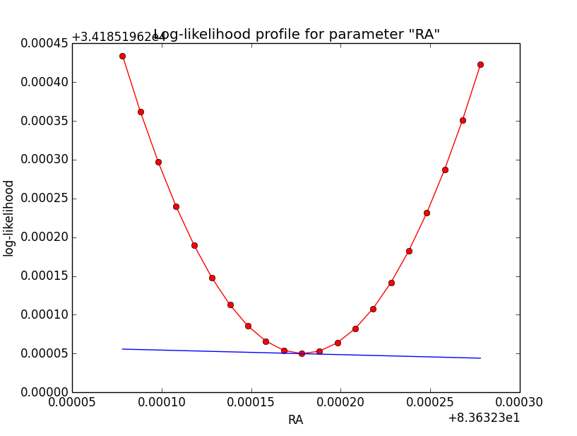
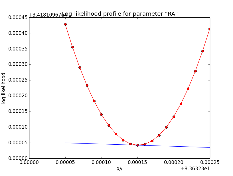
Here a number of log-likelihood profiles for the disk parameters RA (top), DEC (middle), and Radius (bottom). The plots from the left to the right show successive zooms with step size 1e-3 (left), 1e-4 (centre) and 1e-5 (right). The red line connects the computed log-likelihood values (red dots), the blue line indicates the gradient obtained by the optimizer. For gradient computation, a step size of 1e-5 has been used. Obviously, the log-likelihood profile is “nice” at a scale of 1e-3, becomes distorted at a scale of 1e-4 and becomes very noisy at a scale of 1e-5.
 |
 |
 |
 |
 |
 |
 |
 |
 |
#4
Updated by Knödlseder Jürgen over 10 years ago
- Status changed from New to In Progress
- Assigned To set to Knödlseder Jürgen
Reducing the numerical differentiation step-size did not really change anything. So although the profile looks smooth on a large scale, it is not precise enough for accurate numerical derivatives that let the algorithm converge properly.
#5
Updated by Knödlseder Jürgen over 10 years ago
- File disk_unbin_Npred_DEC.png added
- File disk_unbin_Npred_RA.png added
- File disk_unbin_Npred_Radius.png added
- % Done changed from 0 to 10
Npred computation not the problem
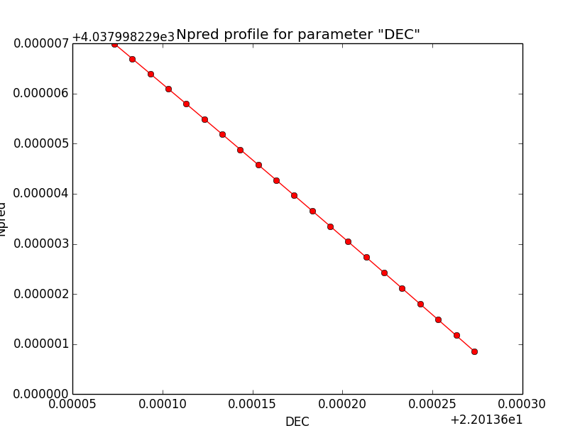
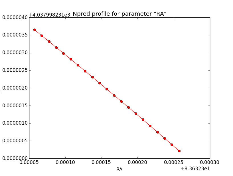
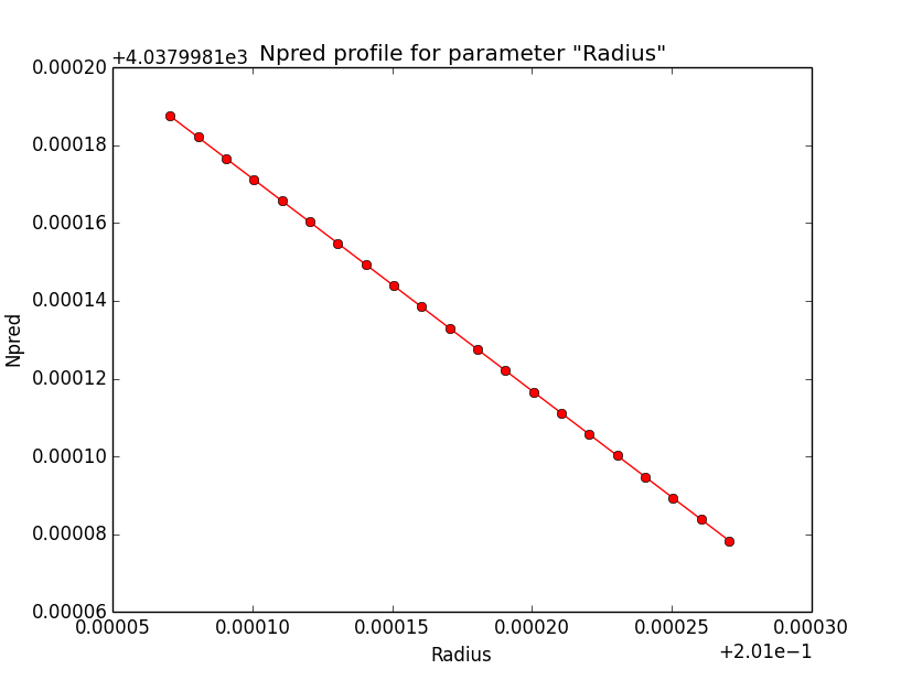
I checked that the Npred term is not the problem in the unbinned analysis. Below are Npred profiles for a step size of 1e-5 in all three parameters. Everything is smooth. This implies that it must be the probability density computation for the individual events that creates the structure in the log-likelihood profiles.
 |
 |
 |
#6
Updated by Knödlseder Jürgen over 10 years ago
Strange: reducing the integration precision improves things
The event probability computation is done in a system centred on the radial model that is integrated radially and azimuthally (in a spherical system). The integration precisions in both dimensions has been set to 1e-5. I reduced the precision to 1e-2, which gave the following result:
>Iteration   0: -logL=34178.844, Lambda=1.0e-03
>Iteration   1: -logL=34176.559, Lambda=1.0e-03, delta=2.285, max(|grad|)=20.694989 [DEC:1]
>Iteration   2: -logL=34176.548, Lambda=1.0e-04, delta=0.011, max(|grad|)=6.348015 [RA:0]
>Iteration   3: -logL=34176.547, Lambda=1.0e-05, delta=0.000, max(|grad|)=-1.458495 [RA:0]
>Iteration   4: -logL=34176.547, Lambda=1.0e-06, delta=0.000, max(|grad|)=0.392503 [RA:0]
>Iteration   5: -logL=34176.547, Lambda=1.0e-07, delta=0.000, max(|grad|)=-0.073415 [RA:0]
 Iteration   6: -logL=34176.547, Lambda=1.0e-08, delta=-0.000, max(|grad|)=0.016422 [RA:0] (stalled)
 Iteration   7: -logL=34176.547, Lambda=1.0e-07, delta=-0.000, max(|grad|)=-0.003630 [RA:0] (stalled)
 Iteration   8: -logL=34176.547, Lambda=1.0e-06, delta=-0.000, max(|grad|)=-0.002001 [Radius:2] (stalled)
 Iteration   9: -logL=34176.547, Lambda=1.0e-05, delta=-0.000, max(|grad|)=0.001361 [Radius:2] (stalled)
 Iteration  10: -logL=34176.547, Lambda=1.0e-04, delta=-0.000, max(|grad|)=0.001189 [Radius:2] (stalled)
>Iteration  11: -logL=34176.547, Lambda=1.0e-03, delta=0.000, max(|grad|)=0.000281 [DEC:1]
=== GObservations ===
 Number of observations ....: 1
 Number of predicted events : 4038
=== GModelSky ===
 Number of spatial par's ...: 3
  RA .......................: 83.6325 +/- 0.00393904 [-360,360] deg (free,scale=1)
  DEC ......................: 22.0138 +/- 0.00327544 [-90,90] deg (free,scale=1)
  Radius ...................: 0.201183 +/- 0.00305945 [0.01,10] deg (free,scale=1)
 Number of spectral par's ..: 3
  Prefactor ................: 5.45629e-16 +/- 1.99354e-17 [1e-23,1e-13] ph/cm2/s/MeV (free,scale=1e-16,gradient)
  Index ....................: -2.45898 +/- 0.0267017 [-0,-5]  (free,scale=-1,gradient)
 === GCTAModelRadialAcceptance ===
  Sigma ....................: 3.05836 +/- 0.0397935 [0.01,10] deg2 (free,scale=1,gradient)
 Number of spectral par's ..: 3
  Prefactor ................: 5.99534e-05 +/- 1.76003e-06 [0,0.001] ph/cm2/s/MeV (free,scale=1e-06,gradient)
  Index ....................: -1.85299 +/- 0.0164762 [-0,-5]  (free,scale=-1,gradient)
This takes less iterations, and the gradients are smaller than initially.
#7
Updated by Knödlseder Jürgen over 10 years ago
- Description updated (diff)
#8
Updated by Knödlseder Jürgen over 10 years ago
- File disk_unbin_scale5_DE_r2a2.png added
- File disk_unbin_scale5_RA_r2a2.png added
- File disk_unbin_scale5_Radius_r2a2.png added
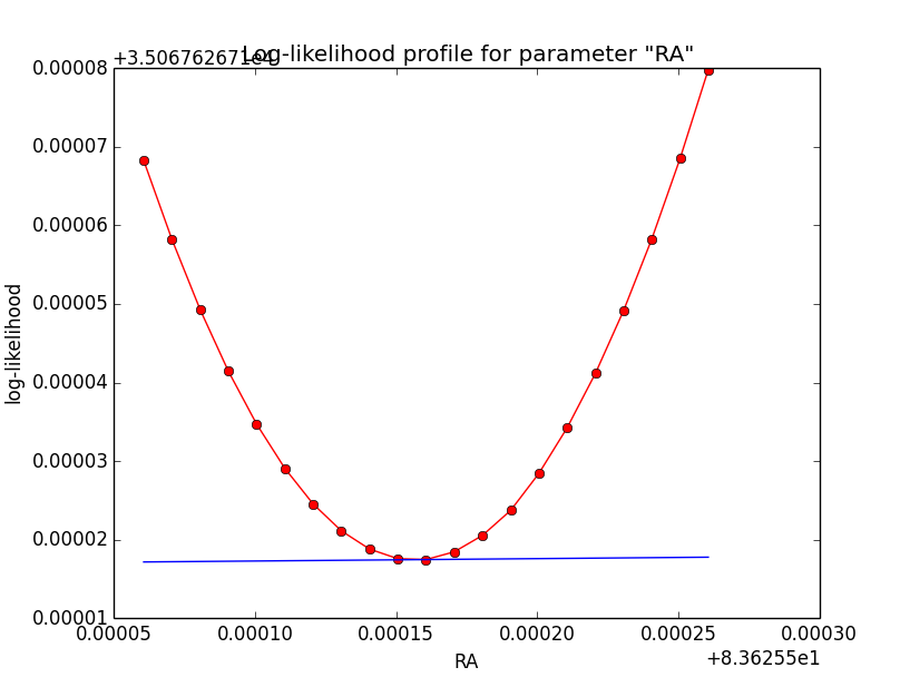
Below the log-likelihood profiles with a step size of 1e-5 for the reduced relative integration precision of 1e-2. This seems counter intuitive, but with less precision the profiles are smoother!
 |
 |
 |
#9
Updated by Knödlseder Jürgen over 10 years ago
- File disk_bin_scale5_Radius_r2a2.png added
- File disk_bin_scale5_RA_r2a2.png added
- File disk_bin_scale5_DEC_r2a2.png added
Binned also better for 1e-2
Here now a comparison of the binned analysis, first with the old precision of 1e-5, and then with the new precision of 1e-2. The fit obviously converges much faster and smoother with the reduced integration precision of 1e-2. The results are pretty much the same.
Integration precision 1e-5
>Iteration   0: -logL=18456.210, Lambda=1.0e-03
>Iteration   1: -logL=18452.575, Lambda=1.0e-03, delta=3.635, max(|grad|)=-28.343815 [RA:0]
>Iteration   2: -logL=18452.529, Lambda=1.0e-04, delta=0.045, max(|grad|)=-16.720985 [DEC:1]
>Iteration   3: -logL=18452.529, Lambda=1.0e-05, delta=0.000, max(|grad|)=6.820850 [DEC:1]
>Iteration   4: -logL=18452.528, Lambda=1.0e-06, delta=0.001, max(|grad|)=-2.600544 [RA:0]
 Iteration   5: -logL=18452.528, Lambda=1.0e-07, delta=-0.000, max(|grad|)=3.205072 [RA:0] (stalled)
 Iteration   6: -logL=18452.528, Lambda=1.0e-06, delta=-0.000, max(|grad|)=3.205211 [RA:0] (stalled)
 Iteration   7: -logL=18452.528, Lambda=1.0e-05, delta=-0.000, max(|grad|)=3.205105 [RA:0] (stalled)
 Iteration   8: -logL=18452.528, Lambda=1.0e-04, delta=-0.000, max(|grad|)=3.204754 [RA:0] (stalled)
 Iteration   9: -logL=18452.528, Lambda=1.0e-03, delta=-0.000, max(|grad|)=3.248355 [RA:0] (stalled)
 Iteration  10: -logL=18452.528, Lambda=1.0e-02, delta=-0.000, max(|grad|)=3.240016 [RA:0] (stalled)
 Iteration  11: -logL=18452.528, Lambda=1.0e-01, delta=-0.000, max(|grad|)=3.080144 [RA:0] (stalled)
>Iteration  12: -logL=18452.528, Lambda=1.0e+00, delta=0.000, max(|grad|)=-1.595976 [Radius:2]
>Iteration  13: -logL=18452.528, Lambda=1.0e-01, delta=0.000, max(|grad|)=2.660137 [DEC:1]
 Iteration  14: -logL=18452.528, Lambda=1.0e-02, delta=-0.000, max(|grad|)=0.518520 [DEC:1] (stalled)
 Iteration  15: -logL=18452.528, Lambda=1.0e-01, delta=-0.000, max(|grad|)=2.844791 [RA:0] (stalled)
>Iteration  16: -logL=18452.528, Lambda=1.0e+00, delta=0.000, max(|grad|)=2.905791 [RA:0]
 Iteration  17: -logL=18452.528, Lambda=1.0e-01, delta=-0.000, max(|grad|)=-2.042002 [RA:0] (stalled)
 Iteration  18: -logL=18452.528, Lambda=1.0e+00, delta=-0.000, max(|grad|)=-1.560911 [RA:0] (stalled)
>Iteration  19: -logL=18452.528, Lambda=1.0e+01, delta=0.000, max(|grad|)=-2.206019 [DEC:1]
=== GObservations ===
 Number of observations ....: 1
 Number of predicted events : 3687
=== GModelSky ===
 Number of spatial par's ...: 3
  RA .......................: 83.6324 +/- 0.00390577 [-360,360] deg (free,scale=1)
  DEC ......................: 22.0143 +/- 0.00329028 [-90,90] deg (free,scale=1)
  Radius ...................: 0.201591 +/- 0.00304322 [0.01,10] deg (free,scale=1)
 Number of spectral par's ..: 3
  Prefactor ................: 5.41603e-16 +/- 1.98302e-17 [1e-23,1e-13] ph/cm2/s/MeV (free,scale=1e-16,gradient)
  Index ....................: -2.45653 +/- 0.0267726 [-0,-5]  (free,scale=-1,gradient)
=== GCTAModelRadialAcceptance ===
 Number of radial par's ....: 1
  Sigma ....................: 3.15909 +/- 0.0857976 [0.01,10] deg2 (free,scale=1,gradient)
 Number of spectral par's ..: 3
  Prefactor ................: 5.88695e-05 +/- 1.90709e-06 [0,0.001] ph/cm2/s/MeV (free,scale=1e-06,gradient)
  Index ....................: -1.85371 +/- 0.0175121 [-0,-5]  (free,scale=-1,gradient)
Integration precision 1e-2
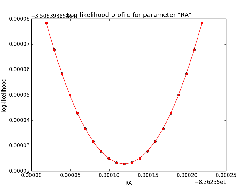
>Iteration   0: -logL=18456.397, Lambda=1.0e-03
>Iteration   1: -logL=18452.583, Lambda=1.0e-03, delta=3.814, max(|grad|)=-20.005022 [RA:0]
>Iteration   2: -logL=18452.538, Lambda=1.0e-04, delta=0.046, max(|grad|)=5.343857 [RA:0]
>Iteration   3: -logL=18452.537, Lambda=1.0e-05, delta=0.000, max(|grad|)=-1.070713 [RA:0]
>Iteration   4: -logL=18452.537, Lambda=1.0e-06, delta=0.000, max(|grad|)=0.358104 [RA:0]
>Iteration   5: -logL=18452.537, Lambda=1.0e-07, delta=0.000, max(|grad|)=0.263873 [Radius:2]
=== GObservations ===
 Number of observations ....: 1
 Number of predicted events : 3687
=== GModelSky ===
 Number of spatial par's ...: 3
  RA .......................: 83.6325 +/- 0.00390558 [-360,360] deg (free,scale=1)
  DEC ......................: 22.0143 +/- 0.00329027 [-90,90] deg (free,scale=1)
  Radius ...................: 0.201619 +/- 0.00304471 [0.01,10] deg (free,scale=1)
 Number of spectral par's ..: 3
  Prefactor ................: 5.39378e-16 +/- 1.97492e-17 [1e-23,1e-13] ph/cm2/s/MeV (free,scale=1e-16,gradient)
  Index ....................: -2.45609 +/- 0.0267721 [-0,-5]  (free,scale=-1,gradient)
=== GCTAModelRadialAcceptance ===
 Number of radial par's ....: 1
  Sigma ....................: 3.15907 +/- 0.0857955 [0.01,10] deg2 (free,scale=1,gradient)
 Number of spectral par's ..: 3
  Prefactor ................: 5.88702e-05 +/- 1.9071e-06 [0,0.001] ph/cm2/s/MeV (free,scale=1e-06,gradient)
  Index ....................: -1.85371 +/- 0.017512 [-0,-5]  (free,scale=-1,gradient)
And here the log-likelihood profiles for binned analysis with an integration precision of 1e-2 at a scale of 1e-5: very smooth!
 |
 |
 |
#10
Updated by Knödlseder Jürgen over 10 years ago
- File gauss_unbin_scale5_RA_r2a2.png added
- File gauss_unbin_scale5_RA_r5a5.png added
- % Done changed from 10 to 20
Gaussian model has problems at all scales!!!
Crosschecking then the unbinned Gaussian model as another case I recognized that also here the log-likelihood profiles are bad, and even for an integration precision of 1e-2 have a kink. Here the iterations of the 1e-5 and 1e-2 precision runs. Fitting results were the same for both runs.
Integration precision 1e-5
>Iteration   0: -logL=35065.905, Lambda=1.0e-03
>Iteration   1: -logL=35062.850, Lambda=1.0e-03, delta=3.055, max(|grad|)=26.700169 [Sigma:2]
>Iteration   2: -logL=35062.829, Lambda=1.0e-04, delta=0.022, max(|grad|)=44.862488 [DEC:1]
 Iteration   3: -logL=35062.829, Lambda=1.0e-05, delta=-0.126, max(|grad|)=-39.775759 [Sigma:2] (stalled)
 Iteration   4: -logL=35062.829, Lambda=1.0e-04, delta=-0.126, max(|grad|)=-39.772432 [Sigma:2] (stalled)
 Iteration   5: -logL=35062.829, Lambda=1.0e-03, delta=-0.126, max(|grad|)=-39.687673 [Sigma:2] (stalled)
 Iteration   6: -logL=35062.829, Lambda=1.0e-02, delta=-0.124, max(|grad|)=-39.369992 [Sigma:2] (stalled)
 Iteration   7: -logL=35062.829, Lambda=1.0e-01, delta=-0.104, max(|grad|)=-71.231283 [Sigma:2] (stalled)
 Iteration   8: -logL=35062.829, Lambda=1.0e+00, delta=-0.039, max(|grad|)=-21.992135 [Sigma:2] (stalled)
 Iteration   9: -logL=35062.829, Lambda=1.0e+01, delta=-0.002, max(|grad|)=-6.135290 [Sigma:2] (stalled)
 Iteration  10: -logL=35062.829, Lambda=1.0e+02, delta=-0.000, max(|grad|)=2.564888 [RA:0] (stalled)
 Iteration  11: -logL=35062.829, Lambda=1.0e+03, delta=-0.000, max(|grad|)=43.240077 [Sigma:2] (stalled)
 Iteration  12: -logL=35062.829, Lambda=1.0e+04, delta=-0.000, max(|grad|)=44.858612 [DEC:1] (stalled)
Integration precision 1e-2
>Iteration   0: -logL=35062.491, Lambda=1.0e-03
>Iteration   1: -logL=35059.403, Lambda=1.0e-03, delta=3.087, max(|grad|)=27.067091 [Sigma:2]
>Iteration   2: -logL=35059.383, Lambda=1.0e-04, delta=0.020, max(|grad|)=-2.179918 [Sigma:2]
>Iteration   3: -logL=35059.383, Lambda=1.0e-05, delta=0.000, max(|grad|)=-0.884052 [RA:0]
 Iteration   4: -logL=35059.383, Lambda=1.0e-06, delta=-0.000, max(|grad|)=0.904869 [RA:0] (stalled)
 Iteration   5: -logL=35059.383, Lambda=1.0e-05, delta=-0.000, max(|grad|)=0.904726 [RA:0] (stalled)
 Iteration   6: -logL=35059.383, Lambda=1.0e-04, delta=-0.000, max(|grad|)=0.904932 [RA:0] (stalled)
 Iteration   7: -logL=35059.383, Lambda=1.0e-03, delta=-0.000, max(|grad|)=0.904089 [RA:0] (stalled)
 Iteration   8: -logL=35059.383, Lambda=1.0e-02, delta=-0.000, max(|grad|)=0.893860 [RA:0] (stalled)
 Iteration   9: -logL=35059.383, Lambda=1.0e-01, delta=-0.000, max(|grad|)=0.803572 [RA:0] (stalled)
>Iteration  10: -logL=35059.383, Lambda=1.0e+00, delta=0.000, max(|grad|)=0.253246 [RA:0]
>Iteration  11: -logL=35059.383, Lambda=1.0e-01, delta=0.000, max(|grad|)=-0.104525 [RA:0]
>Iteration  12: -logL=35059.383, Lambda=1.0e-02, delta=0.000, max(|grad|)=0.079574 [RA:0]
And here the log-likelihood profiles, on the left for a precision of 1e-5, on the right for a precision of 1e-2.
 |
 |
#11
Updated by Knödlseder Jürgen over 10 years ago
Changing the integration scheme does not improve things
I implemented an alternative radial model integration method that uses a coordinate system centred on the Psf instead of the former system that was centred on the model. The integration region is the same, yet once the integration has as symmetry point the Psf centre while in the other case it has the model centre as symmetry point. This may lead to numerically differences.
To check the precision between both computation methods, I computed for the disk model the Irf value for each event with both methods and dumped any difference larger than 1% into the console (I’ve choosen 1% as otherwise I got a quite verbose run). Here the outcome (the fit was done using the model-based integration; the step-size for gradient computation was 2e-4, the precision for integration was set to 1e-6 for both methods):
Psf-based=8.41043e+12; Model-based=8.31804e+12; Psf-Model=9.23986e+10; Psf/Model=1.01111
Psf-based=1.79475e+14; Model-based=1.77137e+14; Psf-Model=2.33874e+12; Psf/Model=1.0132
Psf-based=9.60219e+12; Model-based=9.47734e+12; Psf-Model=1.24851e+11; Psf/Model=1.01317
>Iteration   0: -logL=34182.387, Lambda=1.0e-03
Psf-based=9.51493e+12; Model-based=9.39039e+12; Psf-Model=1.24537e+11; Psf/Model=1.01326
>Iteration   1: -logL=34180.097, Lambda=1.0e-03, delta=2.290, max(|grad|)=23.256112 [DEC:1]
>Iteration   2: -logL=34180.086, Lambda=1.0e-04, delta=0.011, max(|grad|)=6.080755 [RA:0]
>Iteration   3: -logL=34180.086, Lambda=1.0e-05, delta=0.000, max(|grad|)=1.558499 [Radius:2]
>Iteration   4: -logL=34180.086, Lambda=1.0e-06, delta=0.000, max(|grad|)=-0.566938 [Radius:2]
 Iteration   5: -logL=34180.086, Lambda=1.0e-07, delta=-0.000, max(|grad|)=0.183964 [Radius:2] (stalled)
 Iteration   6: -logL=34180.086, Lambda=1.0e-06, delta=-0.000, max(|grad|)=0.183985 [Radius:2] (stalled)
 Iteration   7: -logL=34180.086, Lambda=1.0e-05, delta=-0.000, max(|grad|)=0.183965 [Radius:2] (stalled)
 Iteration   8: -logL=34180.086, Lambda=1.0e-04, delta=-0.000, max(|grad|)=0.183878 [Radius:2] (stalled)
 Iteration   9: -logL=34180.086, Lambda=1.0e-03, delta=-0.000, max(|grad|)=0.183239 [Radius:2] (stalled)
 Iteration  10: -logL=34180.086, Lambda=1.0e-02, delta=-0.000, max(|grad|)=0.176919 [Radius:2] (stalled)
 Iteration  11: -logL=34180.086, Lambda=1.0e-01, delta=-0.000, max(|grad|)=0.119540 [Radius:2] (stalled)
 Iteration  12: -logL=34180.086, Lambda=1.0e+00, delta=-0.000, max(|grad|)=0.153442 [RA:0] (stalled)
 Iteration  13: -logL=34180.086, Lambda=1.0e+01, delta=-0.000, max(|grad|)=-0.149491 [Radius:2] (stalled)
 Iteration  14: -logL=34180.086, Lambda=1.0e+02, delta=-0.000, max(|grad|)=-0.147830 [Radius:2] (stalled)
=== GOptimizerLM ===
 Optimized function value ..: 34180.086
And here the console dump in case that the Psf-based integration was used (the difference with respect to the former is that now the Irf was used from the Psf-based integration, leading to a somewhat different iteration scheme):
Psf-based=8.41043e+12; Model-based=8.31804e+12; Psf-Model=9.23986e+10; Psf/Model=1.01111
Psf-based=1.79475e+14; Model-based=1.77137e+14; Psf-Model=2.33874e+12; Psf/Model=1.0132
Psf-based=9.60219e+12; Model-based=9.47734e+12; Psf-Model=1.24851e+11; Psf/Model=1.01317
>Iteration   0: -logL=34182.431, Lambda=1.0e-03
Psf-based=1.77896e+14; Model-based=1.75561e+14; Psf-Model=2.33491e+12; Psf/Model=1.0133
Psf-based=2.90648e+13; Model-based=2.86749e+13; Psf-Model=3.89811e+11; Psf/Model=1.01359
>Iteration   1: -logL=34180.131, Lambda=1.0e-03, delta=2.300, max(|grad|)=58.238133 [RA:0]
 Iteration   2: -logL=34180.131, Lambda=1.0e-04, delta=-0.017, max(|grad|)=-64.345341 [RA:0] (stalled)
 Iteration   3: -logL=34180.131, Lambda=1.0e-03, delta=-0.017, max(|grad|)=-63.541598 [RA:0] (stalled)
 Iteration   4: -logL=34180.131, Lambda=1.0e-02, delta=-0.016, max(|grad|)=-68.675928 [RA:0] (stalled)
 Iteration   5: -logL=34180.131, Lambda=1.0e-01, delta=-0.016, max(|grad|)=-51.220461 [RA:0] (stalled)
>Iteration   6: -logL=34180.123, Lambda=1.0e+00, delta=0.008, max(|grad|)=-22.486019 [DEC:1]
Psf-based=9.52107e+12; Model-based=9.39527e+12; Psf-Model=1.25801e+11; Psf/Model=1.01339
>Iteration   7: -logL=34180.110, Lambda=1.0e-01, delta=0.013, max(|grad|)=39.522341 [Radius:2]
Psf-based=5.02533e+13; Model-based=4.95867e+13; Psf-Model=6.66573e+11; Psf/Model=1.01344
 Iteration   8: -logL=34180.110, Lambda=1.0e-02, delta=-0.025, max(|grad|)=-42.493911 [Radius:2] (stalled)
 Iteration   9: -logL=34180.110, Lambda=1.0e-01, delta=-0.023, max(|grad|)=-55.226406 [Radius:2] (stalled)
Psf-based=5.0183e+13; Model-based=4.95e+13; Psf-Model=6.82977e+11; Psf/Model=1.0138
Psf-based=5.01623e+13; Model-based=4.94955e+13; Psf-Model=6.66865e+11; Psf/Model=1.01347
>Iteration  10: -logL=34180.107, Lambda=1.0e+00, delta=0.003, max(|grad|)=-54.111179 [DEC:1]
Psf-based=1.77426e+14; Model-based=1.75139e+14; Psf-Model=2.28669e+12; Psf/Model=1.01306
Psf-based=1.86115e+13; Model-based=1.83495e+13; Psf-Model=2.6203e+11; Psf/Model=1.01428
 Iteration  11: -logL=34180.107, Lambda=1.0e-01, delta=-0.031, max(|grad|)=45.835401 [DEC:1] (stalled)
 Iteration  12: -logL=34180.107, Lambda=1.0e+00, delta=-0.017, max(|grad|)=62.316907 [DEC:1] (stalled)
Psf-based=5.01642e+13; Model-based=4.94901e+13; Psf-Model=6.74144e+11; Psf/Model=1.01362
 Iteration  13: -logL=34180.107, Lambda=1.0e+01, delta=-0.020, max(|grad|)=33.570227 [DEC:1] (stalled)
Psf-based=5.01786e+13; Model-based=4.94984e+13; Psf-Model=6.80154e+11; Psf/Model=1.01374
Psf-based=5.0158e+13; Model-based=4.94939e+13; Psf-Model=6.64141e+11; Psf/Model=1.01342
 Iteration  14: -logL=34180.107, Lambda=1.0e+02, delta=-0.004, max(|grad|)=-52.946653 [DEC:1] (stalled)
Psf-based=5.01825e+13; Model-based=4.94998e+13; Psf-Model=6.8269e+11; Psf/Model=1.01379
Psf-based=5.01619e+13; Model-based=4.94953e+13; Psf-Model=6.66588e+11; Psf/Model=1.01347
>Iteration  15: -logL=34180.107, Lambda=1.0e+03, delta=0.000, max(|grad|)=-54.562612 [DEC:1]
Psf-based=5.01787e+13; Model-based=4.94984e+13; Psf-Model=6.80328e+11; Psf/Model=1.01374
Psf-based=5.01582e+13; Model-based=4.94938e+13; Psf-Model=6.64307e+11; Psf/Model=1.01342
...
I cut the output after iteration 15, in total 29 iterations were done. Using the Psf-based integration the maximum gradient is considerably larger. This is a good illustration on how the entire process is influenced by numerical (in)stability.
#12
Updated by Knödlseder Jürgen over 10 years ago
- File no-azimuth-integration.png added
Just a note: for the disk model, the azimuthal integration (using the Psf-based system) can be replaced by an analytical model, at least if Aeff is assumed constant over the Psf. Doing this leads to the same behaviour (see also the log-likelihood plot below). This means that the delta integration should be the culprit ...
 |
#13
Updated by Knödlseder Jürgen over 10 years ago
- File integration-psf.png added
- File integration-model.png added
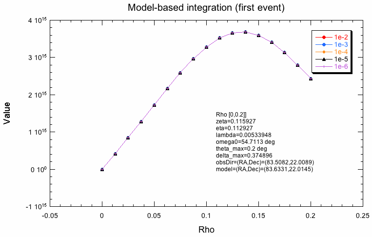
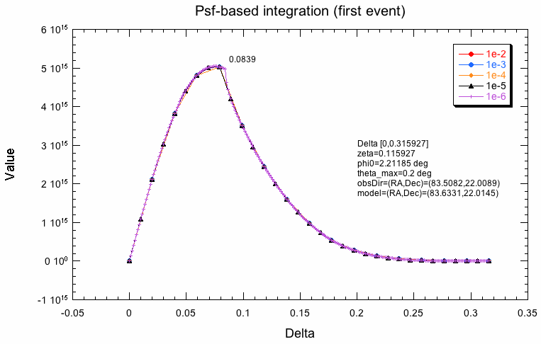
The following plots indicate why the two integration schemes differ. What is shown below is the evaluation of the response along the radial integration direction for the first event in the test dataset for various integration precisions. For model-based integration this is radially outwards from the model centre (coordinate rho), for the Psf-based integration this is radially outwards from the Psf centre (coordinate delta). Obviously, the shape is not the same, which is likely due to the fact that the Psf integration region is larger than the model region. The kink in the Psf-based integration will obviously lead to problems. One can see how the algorithm refines the integration steps with increasing precision, while for the model-based integration, all precisions are reached with the same step size.
 |
 |
#14
Updated by Knödlseder Jürgen over 10 years ago
- File disk_unbin-model_scale5_RA_prec5_grad0002.png added
- File disk_unbin-model-switch_scale5_RA_prec5_grad0002.png added
- % Done changed from 20 to 40
Splitting the integral into two parts
I now implemented a split of the integral into two parts, one to the left and another to the right of the kink (which is fully predictable). Using the model system based integration, an integration precision of 1e-5 and a gradient step size of h=2e-4, I obtained the following log-likelihood profiles (for a step size of 1e-5). Left is before split into two part, right is afterwards. Including the split results in a smoother, though not perfect profile.
 |
 |
It is somehow disappointing that the precision problem of the log-likelihood profile cannot be solved. Globally, the Psf system based integration seems even to be worse that the model system based integration. Somehow the model system based integration kernel seems to be smoother, and thus easier to integrate.
#15
Updated by Knödlseder Jürgen over 10 years ago
Testing a more robust derivative scheme
In case that the log-likelihood profile cannot be made smoother, a more robust numerical derivation scheme is needed. I found this very interesting page web page from Pavel Holoborodko which provides smooth noise-robust differentiators. They require more function evaluations, but overall this may still lead to a gain in computation speed if less iterations would be needed. I played around with a couple of the different schemes, characterized by a degree and a filter length. Below some results for an unbinned analysis. N/A in the degree and filter length column refer to the original difference method.
| Model | Degree | Filter length | Precision | Step size | Iterations | Max. gradient |
| Disk | N/A | N/A | 1e-5 | 2e-4 | 15 | 1.380502 [RA:0] |
| 2 | 5 | 1e-5 | 2e-4 | 16 | 0.405655 [RA:0] | |
| 2 | 7 | 1e-5 | 2e-4 | 8 | 0.000851 [RA:0] | |
| 4 | 7 | 1e-5 | 2e-4 | 13 | 0.606999 [RA:0] | |
| 2 | 5 | 1e-5 | 1e-5 | 12 | -4.197968 [Radius:2] | |
| N/A | N/A | 1e-5 | 1e-3 | 14 | -0.115223 [Radius:2] | |
| 2 | 5 | 1e-5 | 1e-3 | 6 | -0.062993 [RA:0] | |
| 2 | 7 | 1e-5 | 1e-3 | 17 | 0.122399 [RA:0] | |
| 2 | 5 | 1e-2 | 1e-3 | 7 | -0.004124 [RA:0] | |
| N/A | N/A | 1e-2 | 1e-3 | 13 | 2.470741 [Radius:2] | |
| Gauss | N/A | N/A | 1e-5 | 1e-3 | ||
| 2 | 5 | 1e-5 | 1e-3 | 10 | -0.501377 [RA:0] | |
| 2 | 7 | 1e-5 | 1e-3 | 18 | 0.166057 [DEC:1] | |
| 2 | 9 | 1e-5 | 1e-3 | 18 | -0.169905 [RA:0] | |
| 2 | 5 | 1e-2 | 1e-3 | 4 | -0.024501 [Sigma:2] | |
| N/A | N/A | 1e-2 | 1e-3 | 21 | 64.872221 [Sigma:2] | |
| Shell | N/A | N/A | 1e-2 | 1e-3 | ||
| 2 | 5 | 1e-2 | 1e-3 | 32 | 25445.758402 [Radius:2] | |
| 2 | 5 | 1e-5 | 1e-3 | 26 | 25723.513680 [Radius:2] |
There is a trend of smaller maximum gradients with the noise-robust derivatives, in particular for larger filter lengths. However, the only thing that really helps - at least for the disk and the Gaussian model - is setting the integration precision to 1e-2, which now gives very smooth log-likelihood profiles (the kinks shown above for the Gaussian model disappeared after introducing the split integration intervals). Then, the noise-robust estimator with a degree of 2 and a filter length of 5 does a good job.
For the shell, however, nothing seems really to work  The maximum likelihood is probably not reached.
#16
Updated by Knödlseder Jürgen over 10 years ago
- File gauss_5iter.png added
- File gauss_6iter.png added
- File gauss_7iter.png added
- File disk_7iter_prec5-diff.png added
- File disk_6iter_prec5-diff.png added
- File disk_5iter_prec5-diff.png added
Issue solved?
Thinking again over it, I’m wondering whether the “noise” may not come from the fact that the integration precision is not guaranteed. All numerical integration methods do some iterative value refinement, and stop when the difference between subsequent iterations falls below a limit. This may lead to different numbers of iterations depending on details of the setup. When now a parameter is varied, the number of iterations may change, leading to a different value at the end.
I checked this idea using the gauss model, unbinned analysis and model system based integration. For a precision of 1e-2, all rho integrations needed 5 iterations, while for a precision of 1e-5 the number of iterations varied between 5 and 7. The calculations were done using the (2,5) noise-robust derivatives for a step-size h=1e-3.
| Integration iterations | Fit iterations | logL | Max. gradient |
| 5 | 4 | 35067.627 | -0.028632 [Sigma:2] |
| 6 | 6 | 35063.939 | -0.000331 [Sigma:2] |
| 7 | 6 | 35062.852 | -0.000313 [Sigma:2] |
Here the corresponding log-likelihood profiles (from 5 iterations on the left to 7 iterations on the right):
 |
 |
 |
Now the same using the simple difference derivatives for a step-size of h=1e-5.
| Integration iterations | Fit iterations | logL | Max. gradient |
| 5 | 5 | 35067.627 | 0.003536 [Sigma:2] |
| 6 | 4 | 35063.939 | -0.026879 [Sigma:2] |
| 7 | 4 | 35062.852 | -0.025805 [Sigma:2] |
This looks pretty good. Good a quick convergence even for h=1e-5. Now the same (simple difference derivatives, step-size of h=1e-5) for the disk model:
| Integration iterations | Fit iterations | logL | Max. gradient |
| 5 | 5 | 34185.196 | -0.058426 [RA:0] |
| 6 | 5 | 34181.097 | -0.073399 [RA:0] |
| 7 | 5 | 34180.021 | -0.071788 [RA:0] |
 |
 |
 |
For shell models there is still an issue to be solved ...
Conclusion: iterative numerical integration methods with uncontrolled iterations depth are not suited for subsequent numerical differentiation. If numerical derivatives are needed, keep the iterations identical.
#17
Updated by Knödlseder Jürgen over 10 years ago
- File disk_psf-switch_5iter_prec5-diff.png added
Still some trouble with Psf system based integration
I now checked the same philosophy for the Psf system based integration. I started with the disk model.
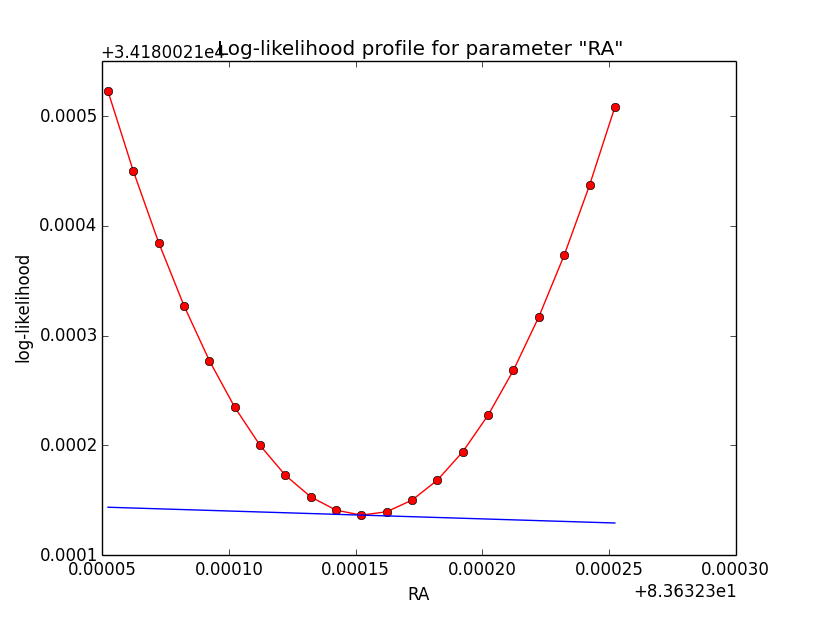
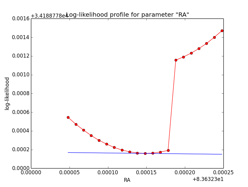
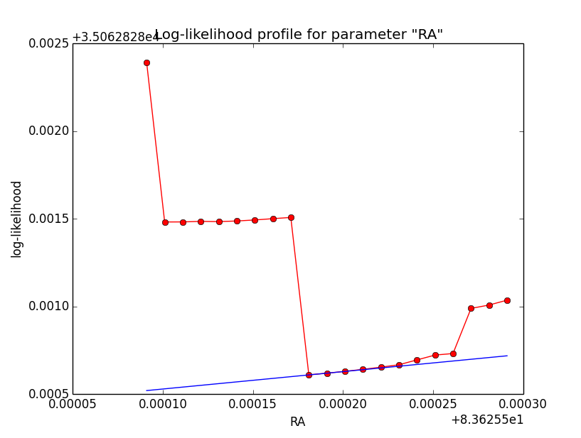
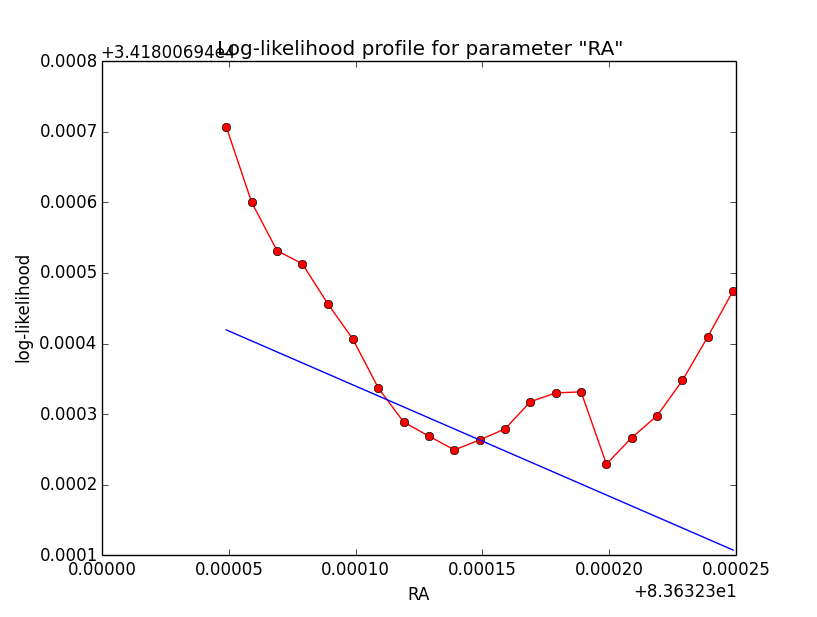
It turns out that with Psf system based integration there is still a problem: the log-likelihood profile is now smooth, but there appears a clear step near the minimum in the profile (see left plot below for 5 iterations). This step changes (see right plot for 8 iterations) with an increasing number of iterations for the integration. This could indicate that the step is related to the limited precision of the integration.
As with the change of the parameters the switch point between full and partial containment of the model within the Psf is changing, the function evaluation in the left and right part of the switch point changes, being a source for discontinuities (as every side will have it’s own intrinsic precision).
| Integration iterations | Fit iterations | logL | Max. gradient |
| 5 | 20 | 34188.778 | 0.493484 [Radius:2] |
| 6 | 18 | 34181.029 | 36.308235 [Radius:2] |
| 8 | 5 | 34180.081 | 0.073235 [Radius:2] |
 |
 |
#18
Updated by Knödlseder Jürgen over 10 years ago
- File disk_psf-switch_8iter_prec5-diff.png added
#19
Updated by Knödlseder Jürgen over 10 years ago
- % Done changed from 40 to 50
Testing the Psf system based on a model that has a radius larger than the Psf radius, and consequently that has no switch points, shows that the problem indeed is related to the switch-point: without switch-point the log-likelihood profiles are smooth.
The question then arose whether the Model system based integration has the same problem with the switch point. My conclusion is no, since the switch point for a Model system based integration will always be at the tail of the Psf, i.e. in a region where the integral is small. The switch point occurs when the Psf is not fully container in the Model, and this happens first for the tail. In a Psf system based integration, the situation is different as in a disk model the model is high up to the boundary (and the Phi angle is largest at the boundary). Consequently, the switch point is always close to the maximum.
Conclusion: a Psf system based integration has poorer properties due to the occurrence of the switch point at function maximum.
I now switch-off the Psf system based integration for unbinned and binned analysis.
#20
Updated by Knödlseder Jürgen over 10 years ago
- Target version set to 00-09-00
- % Done changed from 50 to 80
The shell model still remains a tricky model to integrate, and so far the code is not yet fully satisfactory. Some more investigations are needed.
For the moment let’s stay with the code as is. Here now a check of the Irf computation for all model types and analysis. I show here the computing time needed to estimate the total number of counts in a model, and in parentheses the relative precision achieved. Results are shown for unbinned, binned and stacked analysis. For unbinned, the Npred methods are tested, for binned, the Irf methods are tested. Hence this provides a complete measure of the computing speed (in seconds) and of the precision ((estimated-expected)/expected) of the CTA response computation. The test is done using the script benchmark_irf_computation.py.
| Model | Unbinned | Binned | Stacked |
| Point | 0.0 (0.3%) | 3.8 (0.8%) | 3.0 (0.8%) |
| Disk | 0.1 (0.4%) | 5.4 (1.3%) | 4.0 (1.1%) |
| Gauss | 0.1 (0.2%) | 18.4 (1.1%) | 10.2 (0.9%) |
| Shell | 0.1 (0.3%) | 7.0 (0.7%) | 5.1 (1.1%) |
| Ellipse | 0.1 (0.1%) | 35.8 (1.0%) | 30.3 (0.6%) |
| Diffuse | 0.2 (-0.5%) | 228.8 (0.0%) | 96.0 (0.5%) |
#21
Updated by Knödlseder Jürgen over 10 years ago
And now a benchmark on all model fits, done using benchmark_ml_fitting.py. This checks whether the gradient computations are okay, and whether the fitting algorithm converges reasonably. Bad convergence is indicated by an excessive number of iterations, and these results are marked in bold in the summary table below. Shown are the elapsed time, the number of iterations needed, the log-likelihood, and the fitted source parameters (given in the order they appear in the model).
Obviously, the shell model needs improvements, as well as the ellipse models. I created issue #1303 to follow-up on the shell model improvement and issue #1304 to follow-up on the ellipse model improvement. Also the stacked analysis for the disk is not yet optimal. This will be tracked by issue #1291. The reason why the diffuse analyses needs so many iterations needs also to be understood (see #1305).
| Model | Unbinned | Binned | Stacked |
| Point | 0.1 sec (4, 33105.355, 6.037e-16, -2.496) | 7.3 sec (4, 17179.086, 5.993e-16, -2.492) | 4.8 sec (4, 17179.081, 5.992e-16, -2.492) |
| Disk | 18.9 sec (5, 34176.549, 83.633, 22.014, 0.201, 5.456e-16, -2.459) | 127.9 sec (5, 18452.537, 83.633, 22.014, 0.202, 5.394e-16, -2.456) |
320.5 sec (30, 18451.250, 83.633, 22.015, 0.199, 5.395e-16, -2.462) |
| Gauss | 20.5 sec (4, 35059.430, 83.626, 22.014, 0.204, 5.374e-16, -2.469) | 690.2 sec (4, 19327.126, 83.626, 22.014, 0.205, 5.346e-16, -2.468) | 344.0 sec (4, 19327.270, 83.626, 22.014, 0.205, 5.368e-16, -2.473) |
| Shell | 118.9 sec (30, 35257.950, 83.632, 22.020, 0.281, 0.125, 5.844e-16, -2.449) | 1509.9 sec (36, 19301.494, 83.633, 22.019, 0.289, 0.113, 5.787e-16, -2.447) | 770.5 sec (34, 19301.186, 83.632, 22.021, 0.285, 0.118, 5.798e-16, -2.452) |
| Ellipse | 151.9 sec (32, 35349.603, 83.626, 21.998, 44.725, 0.497, 1.994) | 14291.3 sec (46, 19946.631, 83.627, 22.011, 44.980, 0.482, 1.940, 5.351e-16, -2.487) | - not finished - |
| Diffuse | 1.4 sec (20, 32629.408, 5.299e-16, -2.672) | 5792.3 sec (22, 18221.679, 5.688e-16, -2.657) | 118.8 sec (25, 18221.814, 5.614e-16, -2.670) |
#22
Updated by Knödlseder Jürgen over 10 years ago
- Status changed from In Progress to Closed
- % Done changed from 80 to 100
Close now since follow-up actions have been identified.