Action #1291

Finish implementation of stacked cube analysis
| Status: | Closed | Start date: | 07/23/2014 | |
|---|---|---|---|---|
| Priority: | High | Due date: | ||
| Assigned To: |  Knödlseder Jürgen Knödlseder Jürgen | % Done: | 100% | |
| Category: | - | |||
| Target version: | 00-09-00 | |||
| Duration: |
Description
The stacked cube analysis has been implemented, but support for extended and diffuse models is still lacking in GCTAResponseCube. This issue is to not forget about that, and to fully implement the analysis support.
radio_map.png (54.2 KB)
radio_map_lin.png (42.4 KB)
ptsrc_cube_ra_scale4.png (39.7 KB)
ptsrc_cube_ra_scale5.png (47.2 KB)
ptsrc_cube_ra_scale6.png (50.6 KB)
ptsrc_cube_ra_scale7.png (53.7 KB)
ptsrc_bin_ra_scale4.png (39.1 KB)
ptsrc_bin_ra_scale5.png (43.6 KB)
ptsrc_bin_ra_scale6.png (45.9 KB)
ptsrc_bin_ra_scale7.png (39.5 KB)
ptsrc_bin_ra_scale8.png (41.6 KB)
ptsrc_unbin_ra_scale4.png (39.5 KB)
ptsrc_unbin_ra_scale5.png (46.5 KB)
ptsrc_unbin_ra_scale6.png (36.9 KB)
ptsrc_unbin_ra_scale7.png (45.9 KB)
ptsrc_unbin_ra_scale8.png (34.6 KB)
ptsrc_unbin_ra_scale9.png (37.4 KB)
ptsrc_cube_ra_scale8.png (40.8 KB)
ptsrc_cube_ra_scale9.png (42.3 KB)
ptsrc_bin_ra_scale9.png (47.9 KB)
ptsrc_unbin_ra_scale5_max10.png (43.6 KB)
psf_2D_offset.png (28.6 KB)
psf_2D_original.png (29.1 KB)
psf_king_original.png (27.7 KB)
psf_king_rampdown.png (27.9 KB)
psf_perf_offset.png (26.1 KB)
psf_perf_original.png (26 KB)
ptsrc_cube_scale4_200sqrt.png (39.5 KB)
ptsrc_cube_scale5_200sqrt.png (46.2 KB)
ptsrc_cube_scale6_200sqrt.png (42.8 KB)
logL_king_original.png (37.9 KB)
logL_king_rampdown.png (37.3 KB)


Recurrence
No recurrence.
Related issues
History
#1
 Updated by Knödlseder Jürgen over 10 years ago
- % Done changed from 0 to 10
The actual implementation of the IRF computation in GCTAResponseCube::irf_diffuse is still missing, yet we have the structure in place that allows not handling of the diffuse response cubes. We essentially need now a method that computes the diffuse IRF for a given event.
#2
Updated by Knödlseder Jürgen over 10 years ago
- % Done changed from 10 to 20
I finished the implementation of the diffuse model handling. This required an integration of the diffuse map over the point spread function. Integration is done numerically (as usual), and below I summarize some tests that I did in order to set the integration precision. The column eps(delta) gives the precision for the PSF offset angle integration, the column eps(phi) for the azimuth angle integration. For the latter I tested a dynamic scheme that gives higher precision for small deltas.
The first line gives for comparison the results without integrating the map over the PSF (just taking the map value at the measured event direction). Omitting the PSF integration brings of course a considerable speed increase, but definitely this is not the right thing to do. Nevertheless, the impact on the fitted spectral parameters is not dramatic. Note that the total number of events in the counts cube is 3213.
| eps(delta) | eps(phi) | CPU time (sec) | logL | Iterations | Npred | Prefactor | Index |
| - | - | 19.405 | 18221.640 | 27 | 3213 | 5.509e-16 | -2.660 |
| 1e-4 | 1e-4 | 660.349 | 18221.665 | 38 | 5.657e-16 | -2.671 | |
| 1e-4 | 1e-3 ⇒ 1e-4 | 569.946 | 18221.662 | 38 | 5.658e-16 | -2.671 | |
| 1e-4 | 1e-2 ⇒ 1e-4 | 565.404 | 18221.662 | 38 | 5.658e-16 | -2.671 | |
| 1e-3 | 1e-2 ⇒ 1e-4 | 337.136 | 18221.705 | 38 | 5.630e-16 | -2.676 | |
| 1e-2 | 1e-2 ⇒ 1e-4 | 217.096 | 18221.779 | 24 | 3213 | 5.593e-16 | -2.682 |
| 1e-2 | 1e-2 | 216.235 | 18221.779 | 24 | 3213 | 5.593e-16 | -2.682 |
For comparison the unbinned analysis results:
| CPU time (sec) | logL | Iterations | Prefactor | Index |
| 39.339 | 32629.486 | 22 | 5.257e-16 | -2.681 |
I decided to set eps(delta)=1e-2 and eps(phi)=1e-2, which allows for a ctlike fit of a single FoV in 4 minutes.
#3
Updated by Knödlseder Jürgen over 10 years ago
- File radio_map.png added
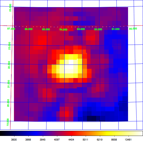
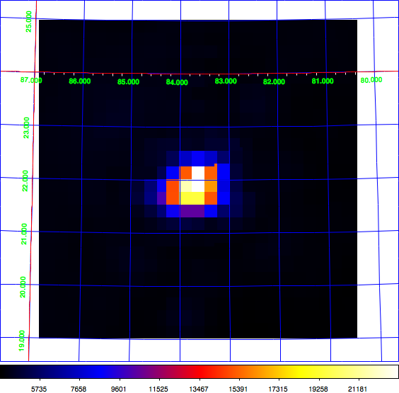
Just for the record: here the diffuse map I use for testing, shown in log scale (left) and linear scale (right). This is a radio map of the Crab region that I now included in the CTA test data. Having a diffuse map of the Crab allows using the same exposure and PSF cube as for the point source analysis.
 |
 |
#4
Updated by Knödlseder Jürgen over 10 years ago
- File radio_map_lin.png added
#5
Updated by Knödlseder Jürgen over 10 years ago
I now start the radial source model part. Here reference values for a Gaussian shaped Crab simulation obtained on my Mac OS X. Binned is extremely slow. The nominal simulated values are given in the table below.
| Parameter | Nominal value |
| RA | 83.6331 |
| Dec | 22.0145 |
| Sigma | 0.2 |
| Prefactor | 5.7e-16 |
| Index | -2.48 |
| Method | CPU time (sec) | logL | Events | Npred | Iterations | Prefactor | Index | RA | Dec | Sigma |
| Unbinned | 84.077 | 35062.787 | 4038 | 4037.98 | 22 | 5.363e-16 | -2.469 | 83.626 | 22.014 | 0.204 |
| Binned | 6974.901 | 19327.144 | 3687 | 3687 | 22 | 5.367e-16 | -2.467 | 83.626 | 22.014 | 0.206 |
#6
Updated by Knödlseder Jürgen over 10 years ago
Here some results for the Gaussian model. Values in parentheses have not been adjusted by the fit (they were not fixed, they just did not move away from the initial location). The integers in parentheses in the eps columns indicate the Romberg order. By default this order is k=5, and I never have touched this before. But it turns out that going from 5 to 3 reduces the average number of function calls from 257 to 21 for a precision of 0.1, one order of magnitude in speed increase (at the expense of reduced precision, though).
| eps(delta) | eps(phi) | CPU (sec) | logL | Iterations | Npred | Prefactor | Index | RA | Dec | Sigma |
| - | - | 11.209 | 19329.790 | 4 | 3687 | 5.132e-16 | -2.460 | (83.6331) | (22.0145) | (0.2) |
| 0.1 (2) | 0.1 (2) | 2663.565 | 19327.298 | 17 (stall) | 3673.37 | 5.220e-16 | -2.472 | 83.626 | 22.008 | 0.203 |
| 0.1 (3) | 0.1 (3) | 523.228 | 19389.287 | 17 (stall) | 3687 | 6.531e-16 | -1.663 | 83.625 | 22.014 | 0.199 |
| 0.1 (4) | 0.1 (3) | 2234.209 | 19328.865 | 36 | 3687.01 | 5.136e-16 | -2.452 | 83.625 | 22.015 | 0.205 |
| 0.1 (5) | 0.1 (3) | 3010.703 | 19327.806 | 28 | 3687.01 | 5.285e-16 | -2.478 | 83.625 | 22.015 | 0.205 |
I implemented an adaptive Simpson’s rule integration in GIntegral. Here some results with that alternative integrator:
| eps(delta) | eps(phi) | CPU (sec) | logL | Iterations | Npred | Prefactor | Index | RA | Dec | Sigma |
| 0.1 | 0.1 | 370.035 | 19389.291 | 12 (stall) | 3687 | 6.536e-16 | -1.663 | 83.625 | 22.014 | 0.199 |
| 0.1 | 0.01 | 1270.653 | 19388.654 | 28 | 3687.1 | 6.539e-16 | -1.669 | 83.624 | 22.012 | 0.199 |
And another method: Gauss-Kronrod integration. I have not yet managed to get meaning results from that.
#7
 Updated by Lu Chia-Chun over 10 years ago
Hi Juergen,
I am interested and want to help, but I really don’t know what you are doing
I even don’t know how you got Cube analysis work....
#8
Updated by Knödlseder Jürgen over 10 years ago
Lu Chia-Chun wrote:
Hi Juergen,
I am interested and want to help, but I really don’t know what you are doing
I even don’t know how you got Cube analysis work....
Thanks for offering help. I’ll look into your background setup problem later. Maybe something is wrong with the units in ctbkgcube, possibly we need to divide by ontime ... need to check.
#9
Updated by Knödlseder Jürgen over 10 years ago
- % Done changed from 20 to 30
Lu Chia-Chun wrote:
Hi Juergen,
I am interested and want to help, but I really don’t know what you are doing
Just to explain: the cube-style analysis needs methods for instrument response function computation that make use of the exposure and PSF cubes. As you recognized, for cube-style analysis there is no pointing. The original analysis was always done in a system centred on the CTA pointing.
The handling of instrument response functions differ for point sources, diffuse sources and radial or elliptical sources. So far I got point source and diffuse map analysis working, currently I’m struggling with the radial and elliptical models. The basic operation that is needed is for each event bin, integration of the model over the PSF. For a point source this is easy, as the model is a Dirac in the sky, hence the integral is just the PSF for the delta value that corresponds to the distance between observed direction and true direction.
For a diffuse model this is also relatively easy, as the shape is fixed, hence you can pre-compute the diffuse model once and then re-use the pre-computed values. This is now also working.
For radial or elliptical models, the issue is that the model can change in each iteration of the fit, so you cannot pre-compute anything. The integration has to be done on-the-fly.
Now I’m currently examining the impact of the requested precision of the integration on CPU time and the fitted results. Asking for poor precision gives a reasonably fast computation, but inaccurate results. I now also started to implement different integration algorithms, yet so far this does also not help. I’m not sure that we can really find a good solution to speed-up things.
#10
Updated by Lu Chia-Chun over 10 years ago
I feel that I won’t be helpful anyway, but one comment: The speed probably doesn’t matter much since the fit process for Cube analysis is relatively short. The only concern regarding the speed is to calculate a TS map, which won’t use varying models except a moving point-like source.
#11
Updated by Knödlseder Jürgen over 10 years ago
As the model computation presents the bottle-neck of the computations, I re-considered the inner loop computations. In fact, the theta angle of the radial model can be obtained using a simple cosine formula, requiring one cos() and one arccos(), one multiplication and one addition in the inner kernel. Here the results using that new method:
Romberg integration:| eps(delta) | eps(phi) | CPU (sec) | logL | Iterations | Npred | Prefactor | Index | RA | Dec | Sigma |
| 0.1 (3) | 0.1 (3) | 163.645 | 19388.742 | 11 | 3687 | 6.694e-16 | -1.664 | 83.625 | 22.012 | 0.201 |
| 0.01 (3) | 0.01 (3) | 1550.499 | 19327.028 | 24 | 3687.05 | 5.345e-16 | -2.474 | 83.625 | 22.013 | 0.207 |
| 0.01 (5) | 0.01 (5) | 1301.864 | 19327.157 | 19 | 3686.89 | 5.286e-16 | -2.478 | 83.626 | 22.014 | 0.205 |
| 0.001 (5) | 0.01 (5) | 1477.916 | 19327.021 | 18 | 3686.93 | 5.286e-16 | -2.473 | 83.625 | 22.014 | 0.205 |
| 0.01 (5) | 0.001 (5) | 1294.381 | 19327.157 | 19 | 3686.89 | 5.286e-16 | -2.478 | 83.626 | 22.014 | 0.205 |
| 0.001 (5) | 0.001 (5) | 1664.157 | 19327.021 | 18 | 3686.93 | 5.286e-16 | -2.473 | 83.625 | 22.014 | 0.205 |
| eps(delta) | eps(phi) | CPU (sec) | logL | Iterations | Npred | Prefactor | Index | RA | Dec | Sigma |
| 0.1 | 0.1 | 3152.350 | 19326.974 | 20 | 3686.97 | 5.288e-16 | -2.469 | 83.625 | 22.014 | 0.205 |
| 0.01 | 0.01 | 4820.155 | 19326.973 | 20 | 3686.97 | 5.288e-16 | -2.469 | 83.625 | 22.014 | 0.205 |
#12
Updated by Knödlseder Jürgen over 10 years ago
Lu Chia-Chun wrote:
I feel that I won’t be helpful anyway, but one comment: The speed probably doesn’t matter much since the fit process for Cube analysis is relatively short. The only concern regarding the speed is to calculate a TS map, which won’t use varying models except a moving point-like source.
Well look at the numbers: for the moment you may wait for 2 hours just for fitting a simple Gaussian-shaped extended source. This was one of the issues raised at the last coding sprint. So I will give it at least a try to see if I can optimize things.
Computing TS maps is likely faster. Some time can be saved in switching off the error computation in the likelihood fit (these are not needed for TS maps, but require some computational time). I created an issue for that (#1294).
#13
Updated by Knödlseder Jürgen over 10 years ago
- http://www.holoborodko.com/pavel/numerical-methods/numerical-integration/cubature-formulas-for-the-unit-disk/
- http://nines.cs.kuleuven.be/ecf/
- http://www.cs.kuleuven.be/publicaties/rapporten/tw/TW300.pdf
#14
Updated by Knödlseder Jürgen over 10 years ago
As the test via model fitting takes too much time, I finally decided to write a specific response computation benchmark that computes the model map for a source model. The script is benchmark_irf_computation.py (once it’s committed The expected number of events for the integration has been estimated using ctobssim to 935.1 +/- 3.1. The first line gives for reference the results for the original binned analysis (which uses a precision of 1e-5 and an order of 5 for the integration in both dimensions).
| Integrator | eps(delta) | eps(phi) | CPU (sec) | Events | Difference | Warnings |
| Romberg (binned) | - | - | 56.833 | 941.393 | 6.293 (0.7%) | no |
| Romberg | 0.01 (2) | 0.01 (2) | 37.215 | 952.017 | 16.917 (1.8%) | no |
| Romberg | 0.01 (3) | 0.01 (3) | 16.485 | 946.195 | 11.095 (1.2%) | no |
| Romberg | 0.01 (4) | 0.01 (4) | 10.549 | 974.960 | 39.860 (4.3%) | no |
| Romberg | 0.01 (5) | 0.01 (5) | 14.889 | 957.905 | 22.805 (2.4%) | no |
| Romberg | 0.01 (6) | 0.01 (6) | 40.791 | 953.926 | 18.826 (2.0%) | no |
| Romberg | 5e-3 (4) | 5e-3 (4) | 11.319 | 964.235 | 29.135 (3.1%) | no |
| Romberg | 5e-3 (5) | 5e-3 (5) | 14.049 | 957.905 | 22.805 (2.4%) | no |
| Romberg | 5e-3 (6) | 5e-3 (6) | 39.690 | 953.926 | 18.826 (2.0%) | no |
| Romberg | 5e-3 (7) | 5e-3 (7) | 133.912 | 954.102 | 19.002 (2.0%) | no |
| Romberg | 1e-3 (3) | 1e-3 (3) | 51.089 | 954.094 | 18.994 (2.0%) | no |
| Romberg | 1e-3 (4) | 1e-3 (4) | 29.956 | 956.970 | 21.870 (2.3%) | no |
| Romberg | 1e-3 (5) | 1e-3 (5) | 17.592 | 955.694 | 20.594 (2.2%) | no |
| Romberg | 1e-3 (6) | 1e-3 (6) | 40.476 | 953.926 | 18.826 (2.0%) | no |
| Romberg | 1e-3 (7) | 1e-3 (7) | 130.903 | 954.102 | 19.002 (2.0%) | no |
| Gauss-Kronrod | 0.01 | 0.01 | 53.695 | 954.117 | 19.017 (2.0%) | no |
| Adaptive Simpson | 0.01 | 0.01 | yes (delta) |
The adaptive Simpson integrator results in many warnings.
#15
Updated by Knödlseder Jürgen over 10 years ago
Now a similar analysis for a disk model. The expected number of events for the integration has been estimated using ctobssim to 933.6 +/- 3.1. The first line gives for reference the results for the original binned analysis (which uses a precision of 1e-5 and an order of 5 for the integration in both dimensions). I only explored values that gave reasonable performance for the Gaussian.
| Integrator | eps(delta) | eps(phi) | CPU (sec) | Events | Difference | Warnings |
| Romberg (binned) | - | - | 9.294 | 942.009 | 8.409 (0.9%) | no |
| Romberg | 0.01 (2) | 0.01 (2) | 65.434 | 955.663 | 22.063 (2.4%) | no |
| Romberg | 0.01 (3) | 0.01 (3) | 26.429 | 966.904 | 33.304 (3.6%) | no |
| Romberg | 0.01 (4) | 0.01 (4) | 12.178 | 971.668 | 38.068 (4.1%) | no |
| Romberg | 0.01 (5) | 0.01 (5) | 5.935 | 959.106 | 25.506 (2.7%) | no |
| Romberg | 0.01 (6) | 0.01 (6) | 7.257 | 954.626 | 21.026 (2.3%) | no |
| Romberg | 0.01 (7) | 0.01 (7) | 17.785 | 954.846 | 21.246 (2.3%) | no |
| Romberg | 5e-3 (6) | 0.01 (6) | 12.101 | 954.626 | 21.026 (2.3%) | no |
| Romberg | 5e-3 (6) | 5e-3 (6) | 13.170 | 954.626 | 21.026 (2.3%) | no |
| Romberg | 1e-3 (2) | 1e-3 (2) | yes (phi) | |||
| Romberg | 1e-3 (3) | 1e-3 (3) | 731.052 | 955.705 | 22.105 (2.4%) | no |
| Romberg | 1e-3 (4) | 1e-3 (4) | 90.514 | 966.427 | 32.827 (3.5%) | no |
| Romberg | 1e-3 (5) | 1e-3 (5) | 33.493 | 965.336 | 31.736 (3.4%) | no |
| Romberg | 1e-3 (6) | 1e-3 (6) | 12.255 | 954.639 | 21.039 (2.3%) | no |
| Romberg | 1e-3 (7) | 1e-3 (7) | 27.319 | 954.846 | 21.246 (2.3%) | no |
| Romberg | 1e-4 (5) | 1e-4 (5) | 476.429 | 955.462 | 21.862 (2.3%) | no |
| Romberg | 1e-4 (6) | 1e-4 (6) | 90.005 | 955.697 | 22.097 (2.4%) | no |
| Gauss-Kronrod | 0.01 | 0.01 | 111.570 | 954.911 | 21.311 (2.3%) | yes (theta,phi) |
| Adaptive Simpson | 0.01 | 0.01 | yes (theta,phi) |
The adaptive Simpson and Gauss-Kronrod integrator results in many warnings. This may be related to discontinuities at the edge of the model.
#16
Updated by Knödlseder Jürgen over 10 years ago
Now a similar analysis for a shell model. The expected number of events for the integration has been estimated using ctobssim to 933.5 +/- 3.1. The first line gives for reference the results for the original binned analysis (which uses a precision of 1e-5 and an order of 5 for the integration in both dimensions). I only explored values that gave reasonable performance for the Gaussian.
| Integrator | eps(delta) | eps(phi) | CPU (sec) | Events | Difference | Warnings |
| Romberg (binned) | - | - | 28.900 | 941.319 | 7.819 (0.8%) | no |
| Romberg | 0.01 (4) | 0.01 (4) | 11.001 | 984.186 | 50.686 (5.4%) | no |
| Romberg | 0.01 (5) | 0.01 (5) | 7.028 | 958.116 | 24.616 (2.6%) | no |
| Romberg | 0.01 (6) | 0.01 (6) | 13.162 | 954.135 | 20.635 (2.2%) | no |
| Romberg | 0.01 (7) | 0.01 (7) | 38.915 | 954.317 | 20.817 (2.2%) | no |
| Romberg | 5e-3 (5) | 5e-3 (5) | 6.819 | 958.209 | 24.709 (2.6%) | no |
| Romberg | 5e-3 (6) | 5e-3 (6) | 14.730 | 954.135 | 20.635 (2.2%) | no |
| Romberg | 5e-3 (7) | 5e-3 (7) | 38.658 | 954.317 | 20.817 (2.2%) | no |
| Romberg | 1e-3 (5) | 1e-3 (5) | 27.542 | 957.005 | 23.505 (2.5%) | no |
| Romberg | 1e-3 (6) | 1e-3 (6) | 14.317 | 954.136 | 20.636 (2.2%) | no |
| Romberg | 1e-3 (7) | 1e-3 (7) | 38.188 | 954.317 | 20.817 (2.2%) | no |
#17
Updated by Knödlseder Jürgen over 10 years ago
Below a summary of the essential results for the Gauss, Disk and Shell models. First row is for original binned analysis.
| eps | order | Gauss | Disk | Shell |
| - | - | 56.8 (0.7%) | 9.3 (0.9%) | 28.9 (0.8%) |
| 0.01 | 5 | 14.9 (2.4%) | 5.9 (2.7%) | 7.0 (2.6%) |
| 0.01 | 6 | 40.8 (2.0%) | 7.3 (2.3%) | 13.1 (2.2%) |
| 5e-3 | 5 | 14.0 (2.4%) | - | 6.8 (2.6%) |
| 5e-3 | 6 | 39.7 (2.0%) | 13.2 (2.3%) | 14.7 (2.2%) |
| 1e-3 | 5 | 17.6 (2.2%) | 33.5 (3.4%) | 27.5 (2.5%) |
| 1e-3 | 6 | 40.5 (2.0%) | 12.3 (2.3%) | 14.3 (2.2%) |
All runs seem to overestimate the total number of counts by about 2%. This is stable with increasing integration precision, and thus is more likely a limit of the exposure or PSF cube computation. Interestingly, this overestimate remains if the number of bins in the PSF cube or the maximum delta angle is increased.
From computation time spent in the calculations, the combination eps=0.01 and order=5 is most interesting. This combination provides a good speed increase with respect to the original binned analysis, while keeping relatively good precision. Better precisions can be achieved with eps=0.001 and order=6, at the expense of an increase computing time. I thus set eps=0.01 and order=5 in the code.
#18
Updated by Knödlseder Jürgen over 10 years ago
- % Done changed from 30 to 50
Here a summary table of the current IRF computation times, obtained using benchmark_irf_computation.py, for original binned analysis and stacked cube analysis. The table gives the CPU time in seconds. In parentheses are the relative differences between IRF computation and ctobssim simulations.
| Model | Binned | Stacked cube |
| Point | 4.118 (0.8%) | 3.139 (1.0%) |
| Gauss | 40.209 (0.7%) | 15.229 (1.2%) |
| Disk | 6.856 (0.9%) | 5.252 (1.5%) |
| Shell | 30.595 (0.8%) | 7.050 (1.4%) |
| Diffuse | 280.794 sec (0.0%) | 226.324 (0.6%) |
The relative differences are now smaller since I managed to fix a bug in the deadtime corrections.
#19
Updated by Knödlseder Jürgen over 10 years ago
Here now an initial try of the elliptical model. Recall that the original binned analysis gives a lot of integration warnings (first row), I thus reduced the precision requirement also for the original binned analysis (second row):
| Integrator | eps(delta) | eps(phi) | CPU (sec) | Events | Difference | Warnings |
| Romberg (binned) | - | - | 61.244 | 854.110 | 8.210 (1.0%) | yes |
| Romberg (binned) | 0.01 | 5 | 42.749 | 854.170 | 8.270 (1.0%) | no |
| Romberg | 0.01 (5) | 0.01 (5) | 56.123 | 854.110 | 8.210 (1.0%) | no |
#20
Updated by Knödlseder Jürgen over 10 years ago
- % Done changed from 50 to 80
I tested the elliptical model computation using stacked cube analysis, and the result was as expected. Looks like I got all the angles right. We’re close of getting this finished 
#21
Updated by Knödlseder Jürgen over 10 years ago
Here the result of a model fit I did using test_binned_ml_fit.py. It took about 4 hours on my Mac OS X! 26 iterations of fitting an ellipse with free position, semiminor and semimajor axes, and positions angle.
The model I injected was the following:
<?xml version="1.0" standalone="no"?>
<source_library title="source library">
  <source name="Gaussian Crab" type="PointSource">
    <spectrum type="PowerLaw">
       <parameter name="Prefactor" scale="1e-16" value="5.7"  min="1e-07" max="1000.0" free="1"/>
       <parameter name="Index"     scale="-1"    value="2.48" min="0.0"   max="+5.0"   free="1"/>
       <parameter name="Scale"     scale="1e6"   value="0.3"  min="0.01"  max="1000.0" free="0"/>
    </spectrum>
    <spatialModel type="EllipticalDisk">
      <parameter name="RA"          scale="1.0" value="83.6331" min="-360"  max="360" free="1"/>
      <parameter name="DEC"         scale="1.0" value="22.0145" min="-90"   max="90"  free="1"/>
      <parameter name="PA"          scale="1.0" value="45.0"    min="-360"  max="360" free="1"/>
      <parameter name="MinorRadius" scale="1.0" value="0.5"     min="0.001" max="10"  free="1"/>
      <parameter name="MajorRadius" scale="1.0" value="2.0"     min="0.001" max="10"  free="1"/>
    </spatialModel>
  </source>
  <source name="Background" type="RadialAcceptance" instrument="CTA">
    <spectrum type="PowerLaw">
       <parameter name="Prefactor" scale="1e-6" value="61.8" min="0.0"  max="1000.0" free="1"/>
       <parameter name="Index"     scale="-1"   value="1.85" min="0.0"  max="+5.0"   free="1"/>
       <parameter name="Scale"     scale="1e6"  value="1.0"  min="0.01" max="1000.0" free="0"/>
    </spectrum>
    <radialModel type="Gaussian">
       <parameter name="Sigma" scale="1.0" value="3.0" min="0.01" max="10.0" free="1"/>
    </radialModel>
  </source>
</source_library>
Here the outcome:
+================================================+
| Stacked maximum likelihood fitting of CTA data |
+================================================+
=== GOptimizerLM ===
 Optimized function value ..: 19947.707
 Absolute precision ........: 1e-06
 Optimization status .......: converged
 Number of parameters ......: 14
 Number of free parameters .: 10
 Number of iterations ......: 26
 Lambda ....................: 1000
=== GObservations ===
 Number of observations ....: 1
 Number of predicted events : 3662.53
=== GCTAObservation ===
 Name ......................:
 Identifier ................:
 Instrument ................: CTA
 Statistics ................: Poisson
 Ontime ....................: 1800 s
 Livetime ..................: 1710 s
 Deadtime correction .......: 0.95
=== GCTAPointing ===
 Pointing direction ........: (RA,Dec)=(83.63,22.01)
=== GCTAResponseCube ===
 Energy dispersion .........: Not used
=== GCTAExposure ===
 Filename ..................: data/expcube.fits
=== GEbounds ===
 Number of intervals .......: 20
 Energy range ..............: 100 GeV - 100 TeV
=== GSkymap ===
 Number of pixels ..........: 2500
 Number of maps ............: 20
 X axis dimension ..........: 50
 Y axis dimension ..........: 50
=== GCTAMeanPsf ===
 Filename ..................: data/psfcube.fits
=== GEbounds ===
 Number of intervals .......: 20
 Energy range ..............: 100 GeV - 100 TeV
 Number of delta bins ......: 60
 Delta range ...............: 0.0025 - 0.2975 deg
=== GSkymap ===
 Number of pixels ..........: 25
 Number of maps ............: 1200
 X axis dimension ..........: 5
 Y axis dimension ..........: 5
=== GCTAEventCube ===
 Number of events ..........: 3666
 Number of elements ........: 800000
 Number of pixels ..........: 40000
 Number of energy bins .....: 20
 Time interval .............: 0 - 1800 sec
=== GModels ===
 Number of models ..........: 2
 Number of parameters ......: 14
=== GModelSky ===
 Name ......................: Gaussian Crab
 Instruments ...............: all
 Instrument scale factors ..: unity
 Observation identifiers ...: all
 Model type ................: ExtendedSource
 Model components ..........: "EllipticalDisk" * "PowerLaw" * "Constant"
 Number of parameters ......: 9
 Number of spatial par's ...: 5
  RA .......................: 83.6283 +/- 0.00685127 [-360,360] deg (free,scale=1)
  DEC ......................: 22.0055 +/- 0.00391877 [-90,90] deg (free,scale=1)
  PA .......................: 45.1424 +/- 0 [-360,360] deg (free,scale=1)
  MinorRadius ..............: 0.493412 +/- 0.00500166 [0.001,10] deg (free,scale=1)
  MajorRadius ..............: 1.90866 +/- 0.014695 [0.001,10] deg (free,scale=1)
 Number of spectral par's ..: 3
  Prefactor ................: 5.35194e-16 +/- 3.28532e-17 [1e-23,1e-13] ph/cm2/s/MeV (free,scale=1e-16,gradient)
  Index ....................: -2.49584 +/- 0.0387742 [-0,-5]  (free,scale=-1,gradient)
  PivotEnergy ..............: 300000 [10000,1e+09] MeV (fixed,scale=1e+06,gradient)
 Number of temporal par's ..: 1
  Constant .................: 1 (relative value) (fixed,scale=1,gradient)
=== GCTAModelRadialAcceptance ===
 Name ......................: Background
 Instruments ...............: CTA
 Instrument scale factors ..: unity
 Observation identifiers ...: all
 Model type ................: "Gaussian" * "PowerLaw" * "Constant"
 Number of parameters ......: 5
 Number of radial par's ....: 1
  Sigma ....................: 3.0136 +/- 0.0823091 [0.01,10] deg2 (free,scale=1,gradient)
 Number of spectral par's ..: 3
  Prefactor ................: 6.23949e-05 +/- 2.38819e-06 [0,0.001] ph/cm2/s/MeV (free,scale=1e-06,gradient)
  Index ....................: -1.8498 +/- 0.0193958 [-0,-5]  (free,scale=-1,gradient)
  PivotEnergy ..............: 1e+06 [10000,1e+09] MeV (fixed,scale=1e+06,gradient)
 Number of temporal par's ..: 1
  Constant .................: 1 (relative value) (fixed,scale=1,gradient)
 Elapsed time ..............: 14945.757 sec
And here a summary of the simulated and fitted parameters:
| Parameter | Simulated | Fitted |
| Prefactor | 5.7e-16 | 5.35194e-16 +/- 3.28532e-17 |
| Index | -2.48 | - 2.49584 +/- 0.0387742 |
| RA | 83.6331 | 83.6283 +/- 0.00685127 |
| Dec | 22.0145 | 22.0055 +/- 0.00391877 |
| PA | 45.0 | 45.1424 +/- 0 |
| MinorRadius | 0.5 | 0.493412 +/- 0.00500166 |
| MajorRadius | 2.0 | 1.90866 +/- 0.014695 |
| Background Prefactor | 6.18e-5 | 6.23949e-05 +/- 2.38819e-06 |
| Background Index | -1.85 | - 1.8498 +/- 0.0193958 |
| Background SIgma | 3.0 | 3.0136 +/- 0.0823091 |
Looks all pretty reasonable. Only the position angle has a zero error (not cleat why). But I need to look into the numerical gradient computation anyhow to see why so many iterations are needed for fitting (which is one of the reasons why this is so time consuming). To do this I should write a script to show a likelihood profile for spatial parameters. This may help to understand whether there is numerical noise, and how the numerical gradient computation can be improved.
#22
Updated by Knödlseder Jürgen over 10 years ago
- File ptsrc_cube_ra_scale4.png added
- File ptsrc_cube_ra_scale5.png added
- File ptsrc_cube_ra_scale6.png added
- File ptsrc_cube_ra_scale7.png added
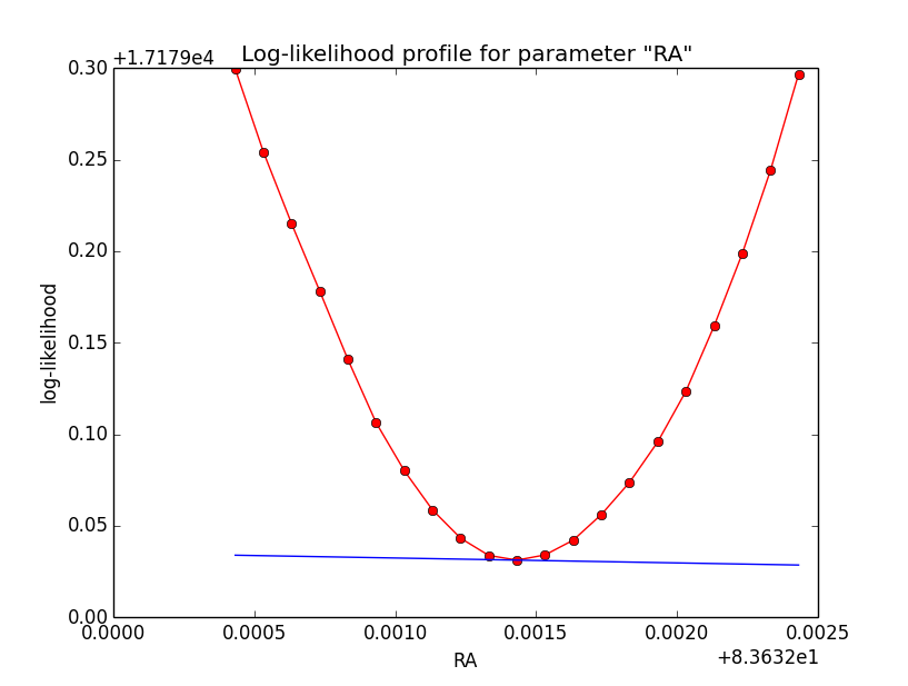
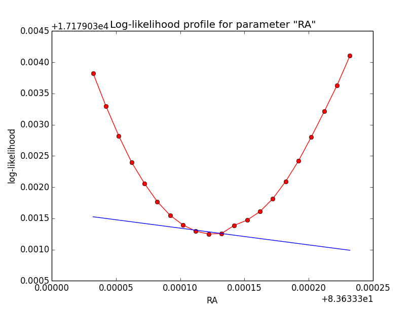
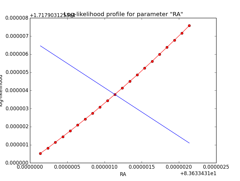
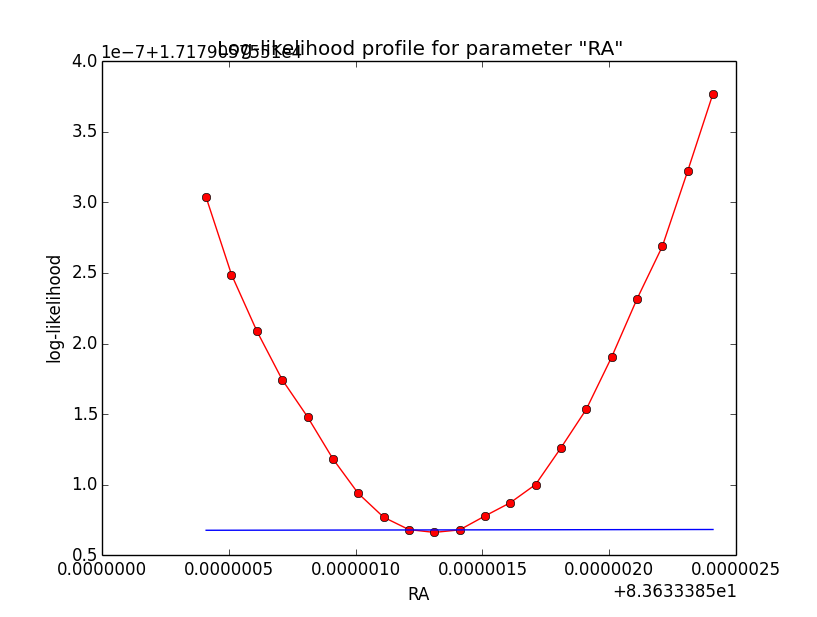
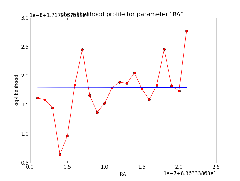
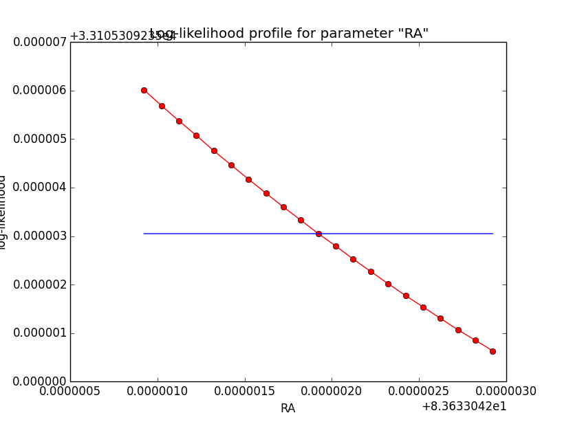
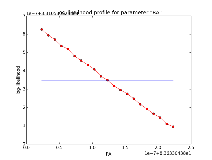
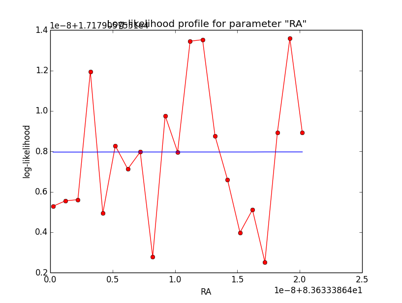
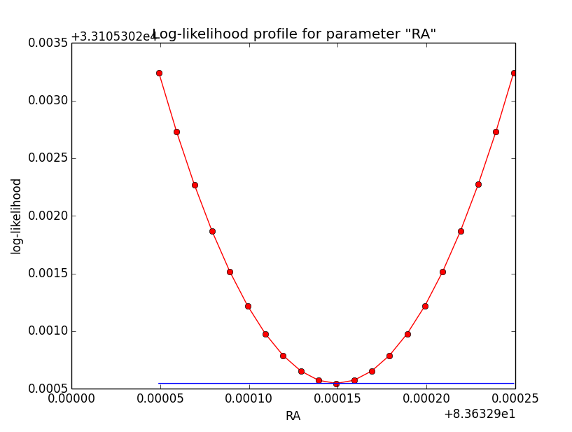
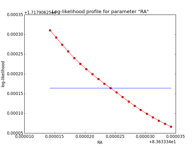
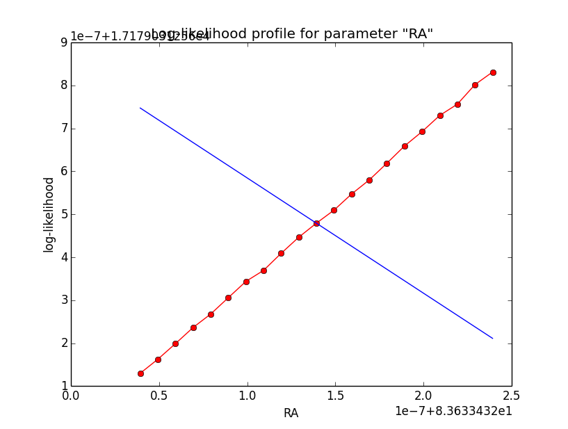
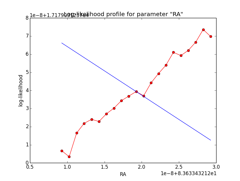
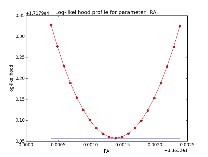
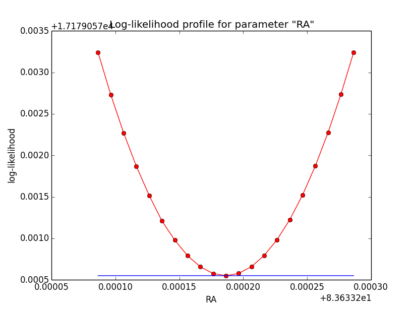
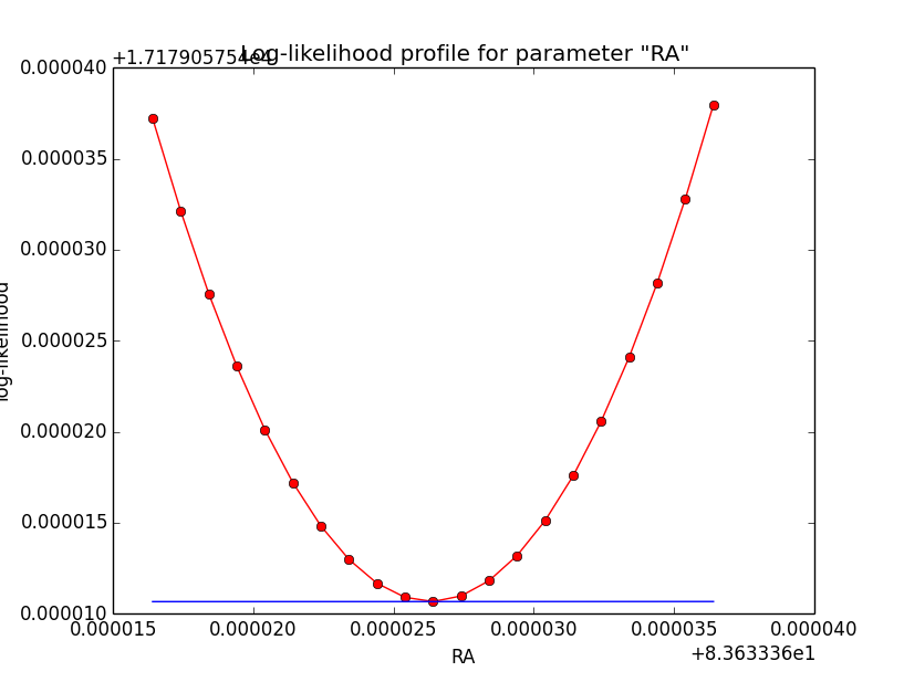
I now looked into the log-likelihood profile of spatial model parameters, starting with the Crab point source fit. I used the script test_likelihood_profile.py for that. I use stacked cube analysis. The optimizer takes 12 iterations and stalls:
=== GOptimizerLM ===
 Optimized function value ..: 17179.031
 Absolute precision ........: 1e-06
 Optimization status .......: stalled
 Number of parameters ......: 11
 Number of free parameters .: 6
 Number of iterations ......: 12
 Lambda ....................: 100000
Below a number of plots that gradually zoom into the profile, which is always centred around the optimum log-likelihood. Step sizes are 1e-4, 1e-5, 1e-6, 1e-7, 1e-8 and , 1e-9. The blue line indicates the gradient estimated by GammaLib. From step size 1e-5 on one sees a clear kink in the profile. The optimum was obviously not found, the gradient is too step. The profile becomes noisy from a step size of 1e-9 on.
 |
 |
 |
 |
 |
 |
#23
Updated by Knödlseder Jürgen over 10 years ago
- File ptsrc_bin_ra_scale4.png added
- File ptsrc_bin_ra_scale5.png added
- File ptsrc_bin_ra_scale6.png added
- File ptsrc_bin_ra_scale7.png added
- File ptsrc_bin_ra_scale8.png added
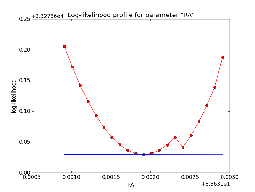
The same now for the original binned analysis. This time, the optimizer converges after 4 iterations. I added one more zoom at 1e-8 to see from which level on the log-likelihood profile becomes irregular.
=== GOptimizerLM ===
 Optimized function value ..: 17179.058
 Absolute precision ........: 1e-06
 Optimization status .......: converged
 Number of parameters ......: 11
 Number of free parameters .: 6
 Number of iterations ......: 4
 Lambda ....................: 1e-07
 |
 |
 |
 |
 |
 |
#24
Updated by Knödlseder Jürgen over 10 years ago
- File ptsrc_unbin_ra_scale4.png added
- File ptsrc_unbin_ra_scale5.png added
- File ptsrc_unbin_ra_scale6.png added
- File ptsrc_unbin_ra_scale7.png added
- File ptsrc_unbin_ra_scale8.png added
- File ptsrc_unbin_ra_scale9.png added
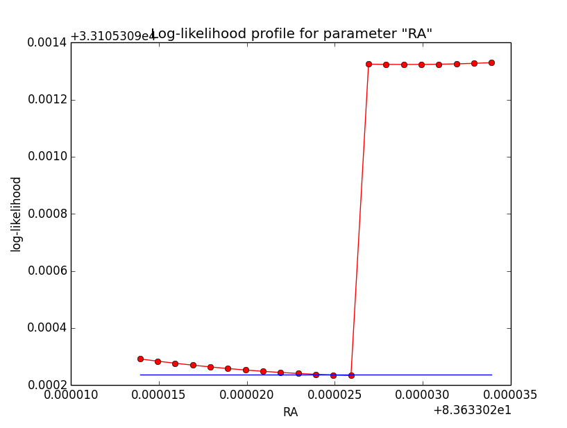
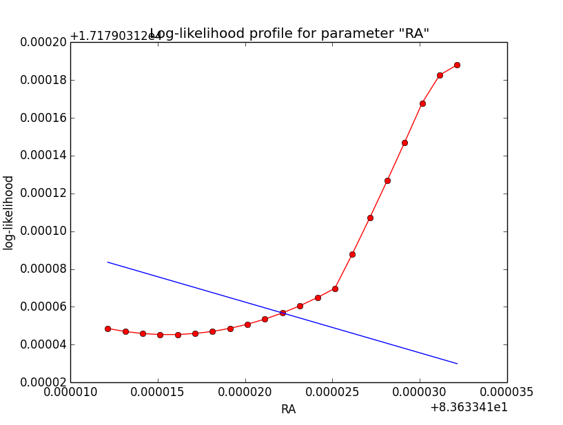
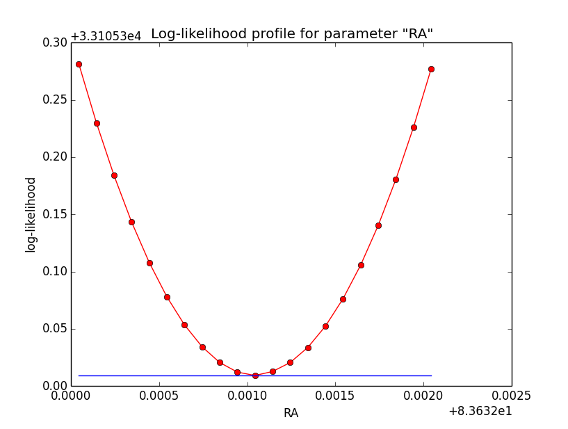
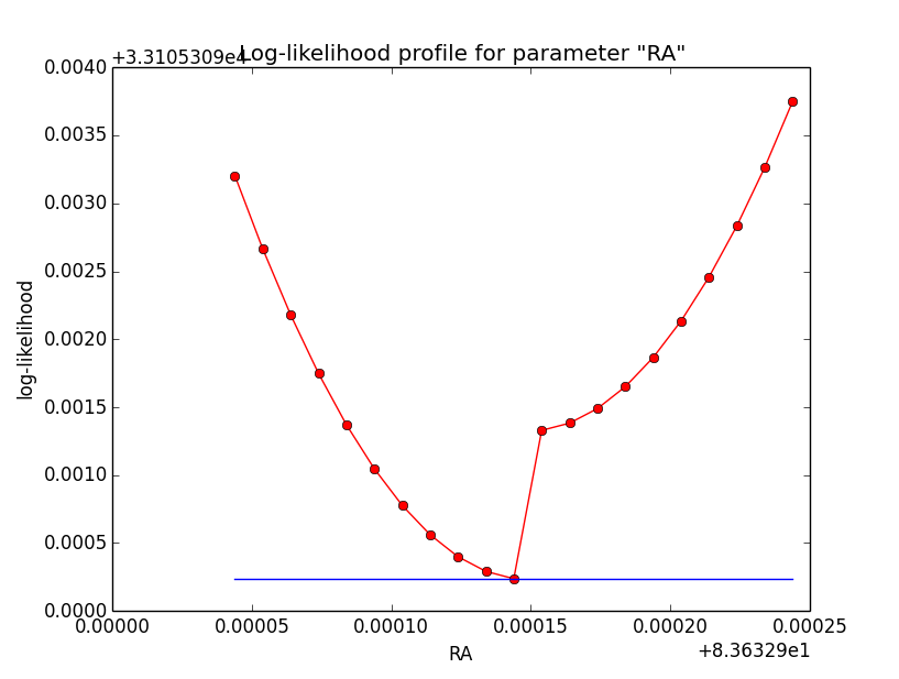
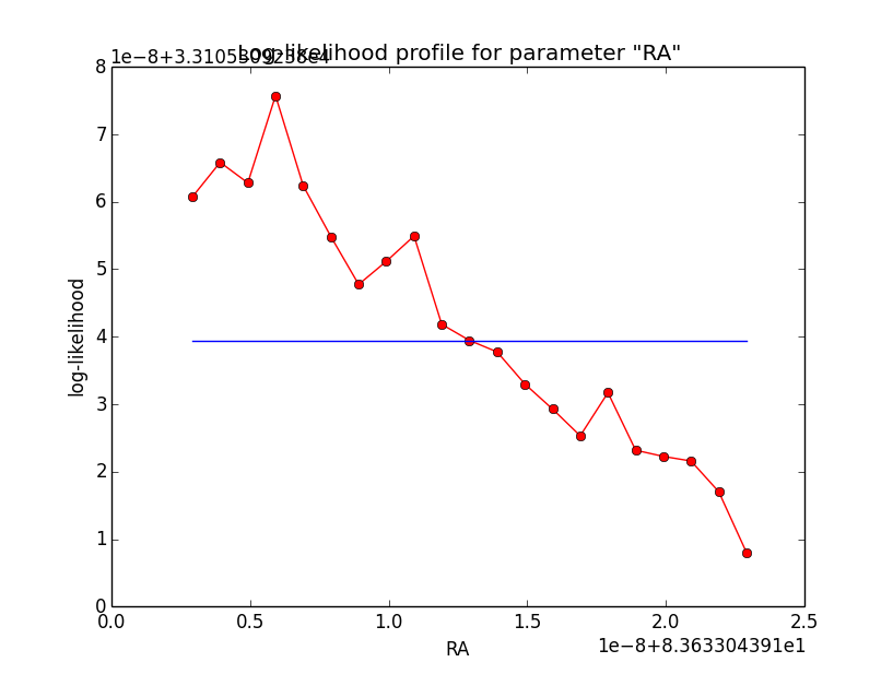
And now the same for unbinned which converged after 6 iterations:
=== GOptimizerLM ===
 Optimized function value ..: 33105.309
 Absolute precision ........: 1e-06
 Optimization status .......: converged
 Number of parameters ......: 11
 Number of free parameters .: 6
 Number of iterations ......: 6
 Lambda ....................: 1e-05
 |
 |
 |
 |
 |
 |
#25
Updated by Knödlseder Jürgen over 10 years ago
- File ptsrc_cube_ra_scale8.png added
- File ptsrc_cube_ra_scale9.png added
#26
Updated by Knödlseder Jürgen over 10 years ago
- File ptsrc_bin_ra_scale9.png added
Conclusion is that numerical noise sets in from a scale of 1e-8 on. More annoying than the numerical noise are the steps in the log-likelihood profiles for unbinned analysis, or the kink for stacked analysis. I was wondering whether this may be related to edge effects of the PSF: the PSF formally drops sharply to zero one delta_max is exceeded.
#27
Updated by Knödlseder Jürgen over 10 years ago
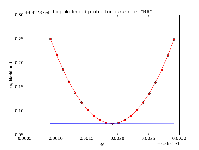
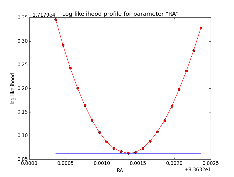
- File ptsrc_unbin_ra_scale5_max10.png added
I increased the delta_max() parameter for the CTA PSF, and indeed, this removed the step from the log-likelihood profile. Below, the comparison of the log-likelihood profile with a step size of 1e-5 for the original delta_max (5 times the Gaussian sigma; left plot) and the increases delta_max (10 times the Gaussian sigma; left plot).
| |
 |
#28
Updated by Knödlseder Jürgen over 10 years ago
- File psf_2D_offset.png added
- File psf_2D_original.png added
- File psf_king_original.png added
- File psf_king_rampdown.png added
- File psf_perf_offset.png added
- File psf_perf_original.png added
- File ptsrc_cube_scale4_200sqrt.png added
- File ptsrc_cube_scale5_200sqrt.png added
- File ptsrc_cube_scale6_200sqrt.png added
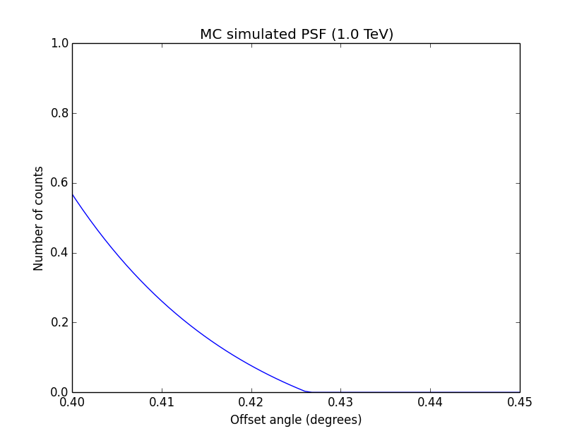
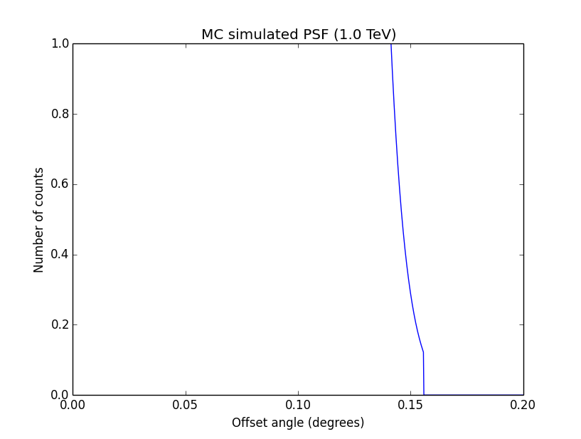
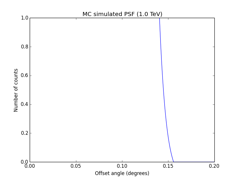
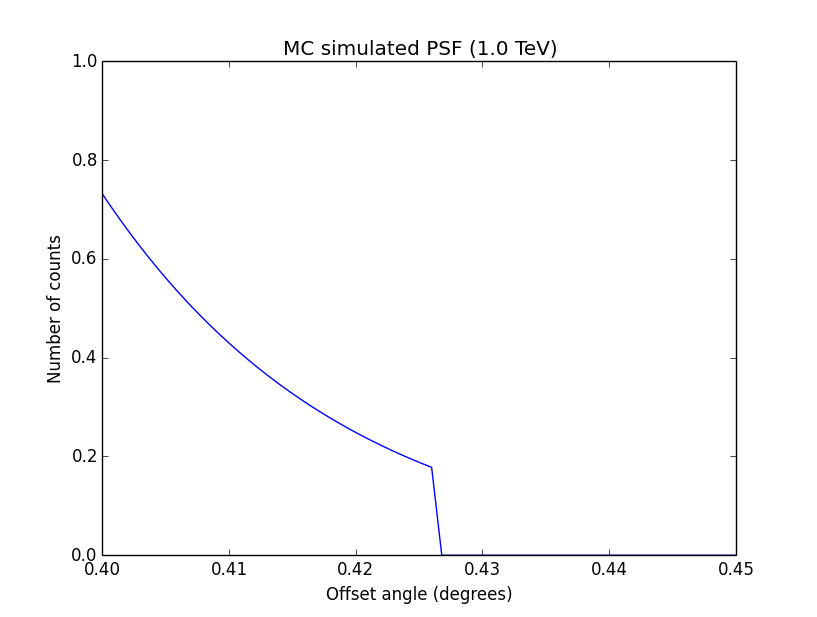
I changed now all response classes to make sure that no discontinuity exists. This removed the steps from the log-likelihood functions. The following plots are for GCTAPsfPerfTable (top), GCTAPsf2D (middle) and GCTAPsfKing (bottom).
 |
 |
 |
 |
 |
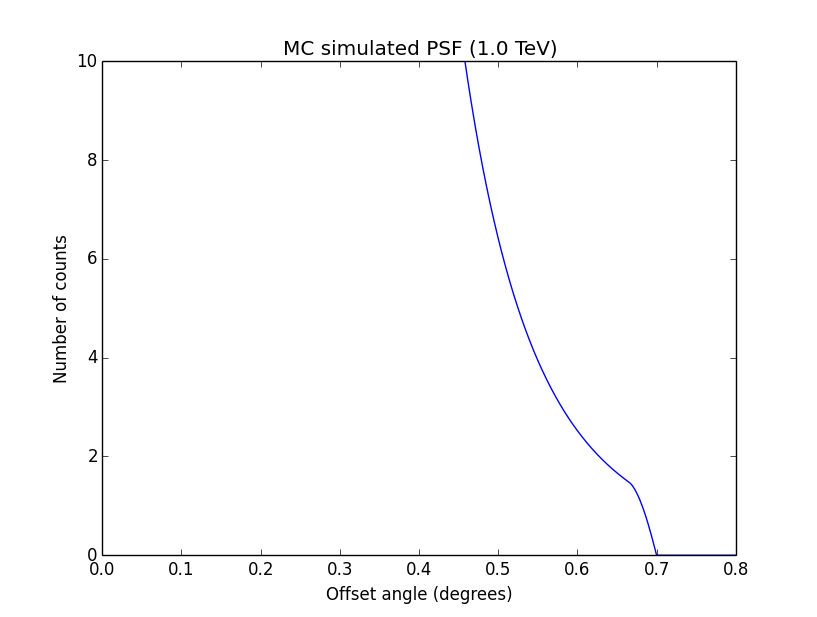 |
Here an example of how the log-likelihood profile improved for the King Psf. Left is original Psf, right is with a rampdown of the Psf at the edge:
 |
 |
Concerning the kink in the stacked cube analysis, this is due to piecewise linear interpolation of the Psf in GCTAMeanPsf. At each delta node, the Psf derivate has a step, which is seen as a kink in the log-likelihood profile. To solve this issue I increases the number of delta bins to 200 (before 60) and I introduced a sqrt sampling that provides a finer node spacing in areas where the Psf is large.
Below the comparison of the old analysis (60 linear bins; top row) to the new analysis (200 sqrt bins; bottom row).
| |
|
|
 |
 |
 |
#29
Updated by Knödlseder Jürgen over 10 years ago
I now looked into the adjustment of the step size in the numerical differentiation in GObservation::model_grad. By default, a step size of h=2e-4 is used, and the gradient is computed using
gradient = ( f(x+h) - f(x-h) ) / ( 2h )I started with the default point source model, the Crab as usual. I only left
RA free, DEC was kept fixed. Here a summary of the runs where I tried different step size of h=1e-5 and h=1e-6:
| Analysis | Step | Iterations | Status | log | RA | Gradient | ||||||||||||||||
| Stacked cube | 2e-4 | 5 | converged | 17179.063 | 83.6334 +/- 0.0014 | 1.86e-5 | |
Stacked cube | 1e-5 | 4 | converged | 17179.063 | 83.6334 +/- 0.0014 | 4.04e-3 | |
Stacked cube | 1e-6 | 5 | converged | 17179.063 | 83.6334 +/- 0.0014 | -2.00 |
The resulting logL and fitted RA parameter & error are always the same. The number of iterations and the resulting gradient differ, though. Below the iteration log for the three cases:
2e-4
>Iteration   0: -logL=17181.880, Lambda=1.0e-03
>Iteration   1: -logL=17179.072, Lambda=1.0e-03, delta=2.808, max(|grad|)=7.809551 [RA:0]
>Iteration   2: -logL=17179.063, Lambda=1.0e-04, delta=0.009, max(|grad|)=0.115662 [Index:8]
>Iteration   3: -logL=17179.063, Lambda=1.0e-05, delta=0.000, max(|grad|)=0.008382 [RA:0]
 Iteration   4: -logL=17179.063, Lambda=1.0e-06, delta=-0.000, max(|grad|)=0.000282 [Index:8] (stalled)
>Iteration   5: -logL=17179.063, Lambda=1.0e-05, delta=0.000, max(|grad|)=0.000019 [RA:0]
1e-5
>Iteration   0: -logL=17181.880, Lambda=1.0e-03
>Iteration   1: -logL=17179.072, Lambda=1.0e-03, delta=2.808, max(|grad|)=-2.312961 [RA:0]
>Iteration   2: -logL=17179.063, Lambda=1.0e-04, delta=0.009, max(|grad|)=0.805540 [RA:0]
>Iteration   3: -logL=17179.063, Lambda=1.0e-05, delta=0.000, max(|grad|)=-0.052719 [RA:0]
>Iteration   4: -logL=17179.063, Lambda=1.0e-06, delta=0.000, max(|grad|)=0.004039 [RA:0]
1e-6
>Iteration   0: -logL=17181.880, Lambda=1.0e-03
>Iteration   1: -logL=17179.072, Lambda=1.0e-03, delta=2.808, max(|grad|)=-1.481153 [Sigma:6]
>Iteration   2: -logL=17179.063, Lambda=1.0e-04, delta=0.009, max(|grad|)=1.815989 [RA:0]
>Iteration   3: -logL=17179.063, Lambda=1.0e-05, delta=0.000, max(|grad|)=-1.869650 [RA:0]
 Iteration   4: -logL=17179.063, Lambda=1.0e-06, delta=-0.000, max(|grad|)=1.940933 [RA:0] (stalled)
>Iteration   5: -logL=17179.063, Lambda=1.0e-05, delta=0.000, max(|grad|)=-2.004162 [RA:0]
For h=1e-6, the gradient oscillates between positive and negative, meaning that the algorithm jumps around the minimum from one side to the other of the log-likelihood function. For h=1e-5 that gradient also oscillates, but becomes smaller. For h=2e-4, the algorithm comes from one side down the hill.
#30
Updated by Knödlseder Jürgen over 10 years ago
Now fitting both RA & DEC:
2e-4
>Iteration   0: -logL=17181.880, Lambda=1.0e-03
>Iteration   1: -logL=17179.042, Lambda=1.0e-03, delta=2.838, max(|grad|)=16.708869 [DEC:1]
>Iteration   2: -logL=17179.032, Lambda=1.0e-04, delta=0.010, max(|grad|)=2.096382 [DEC:1]
>Iteration   3: -logL=17179.032, Lambda=1.0e-05, delta=0.000, max(|grad|)=0.486467 [RA:0]
 Iteration   4: -logL=17179.032, Lambda=1.0e-06, delta=-0.000, max(|grad|)=-0.093080 [RA:0] (stalled)
 Iteration   5: -logL=17179.032, Lambda=1.0e-05, delta=-0.000, max(|grad|)=-0.093072 [RA:0] (stalled)
 Iteration   6: -logL=17179.032, Lambda=1.0e-04, delta=-0.000, max(|grad|)=-0.092985 [RA:0] (stalled)
 Iteration   7: -logL=17179.032, Lambda=1.0e-03, delta=-0.000, max(|grad|)=-0.092504 [RA:0] (stalled)
 Iteration   8: -logL=17179.032, Lambda=1.0e-02, delta=-0.000, max(|grad|)=-0.087291 [RA:0] (stalled)
 Iteration   9: -logL=17179.032, Lambda=1.0e-01, delta=-0.000, max(|grad|)=-0.040023 [RA:0] (stalled)
 Iteration  10: -logL=17179.032, Lambda=1.0e+00, delta=-0.000, max(|grad|)=0.197762 [RA:0] (stalled)
 Iteration  11: -logL=17179.032, Lambda=1.0e+01, delta=-0.000, max(|grad|)=0.434127 [RA:0] (stalled)
 Iteration  12: -logL=17179.032, Lambda=1.0e+02, delta=-0.000, max(|grad|)=0.429050 [RA:0] (stalled)
>Iteration  13: -logL=17179.032, Lambda=1.0e+03, delta=0.000, max(|grad|)=0.428530 [RA:0]
1e-5
>Iteration   0: -logL=17181.880, Lambda=1.0e-03
>Iteration   1: -logL=17179.042, Lambda=1.0e-03, delta=2.838, max(|grad|)=12.188934 [RA:0]
>Iteration   2: -logL=17179.032, Lambda=1.0e-04, delta=0.010, max(|grad|)=0.970879 [RA:0]
>Iteration   3: -logL=17179.032, Lambda=1.0e-05, delta=0.000, max(|grad|)=-0.022085 [RA:0]
>Iteration   4: -logL=17179.032, Lambda=1.0e-06, delta=0.000, max(|grad|)=0.004032 [RA:0]
h=1e-5 behaves definitely better, the gradient decreases while oscillating around the minimum.
#31
Updated by Knödlseder Jürgen over 10 years ago
- File logL_king_original.png added
- File logL_king_rampdown.png added
#32
Updated by Knödlseder Jürgen over 10 years ago
We still need to improve the disk model convergence (see #1299).
#33
Updated by Knödlseder Jürgen about 10 years ago
I made some progress on implementing the elliptical model computations (see #1304) and I now implemented the same logic for the stacked analysis of radial and elliptical models. The main changed for stacked analysis was that I switched from a Psf-based system to a model-based system, as this allows the proper computation of the omega integration range for an elliptical model (and hence allows to implement an analogue code to the one used for unbinned and binned analysis).
Here now as reference the results when running benchmark_ml_fitting.py on the radial disk model using stacked analysis:
>Iteration   0: -logL=18461.345, Lambda=1.0e-03
>Iteration   1: -logL=18455.938, Lambda=1.0e-03, delta=5.407, max(|grad|)=-27.765251 [RA:0]
>Iteration   2: -logL=18455.887, Lambda=1.0e-04, delta=0.051, max(|grad|)=-4.038162 [Radius:2]
 Iteration   3: -logL=18455.887, Lambda=1.0e-05, delta=-0.000, max(|grad|)=-0.842910 [RA:0] (stalled)
 Iteration   4: -logL=18455.887, Lambda=1.0e-04, delta=-0.000, max(|grad|)=-0.842594 [RA:0] (stalled)
 Iteration   5: -logL=18455.887, Lambda=1.0e-03, delta=-0.000, max(|grad|)=-0.839505 [RA:0] (stalled)
 Iteration   6: -logL=18455.887, Lambda=1.0e-02, delta=-0.000, max(|grad|)=-0.808843 [RA:0] (stalled)
>Iteration   7: -logL=18455.887, Lambda=1.0e-01, delta=0.000, max(|grad|)=-0.531971 [RA:0]
=== GOptimizerLM ===
 Optimized function value ..: 18455.887
 Absolute precision ........: 0.001
 Optimization status .......: converged
 Number of parameters ......: 12
 Number of free parameters .: 8
 Number of iterations ......: 7
 Lambda ....................: 0.01
=== GModels ===
 Number of models ..........: 2
 Number of parameters ......: 12
=== GModelSky ===
 Name ......................: Gaussian Crab
 Instruments ...............: all
 Instrument scale factors ..: unity
 Observation identifiers ...: all
 Model type ................: ExtendedSource
 Model components ..........: "DiskFunction" * "PowerLaw" * "Constant"
 Number of parameters ......: 7
 Number of spatial par's ...: 3
  RA .......................: 83.633 +/- 0.0039428 [-360,360] deg (free,scale=1)
  DEC ......................: 22.0141 +/- 0.00331918 [-90,90] deg (free,scale=1)
  Radius ...................: 0.201591 +/- 0.0030387 [0.01,10] deg (free,scale=1)
 Number of spectral par's ..: 3
  Prefactor ................: 5.47633e-16 +/- 2.00549e-17 [1e-23,1e-13] ph/cm2/s/MeV (free,scale=1e-16,gradient)
  Index ....................: -2.415 +/- 0.0268165 [-0,-5]  (free,scale=-1,gradient)
  PivotEnergy ..............: 300000 [10000,1e+09] MeV (fixed,scale=1e+06,gradient)
 Number of temporal par's ..: 1
  Constant .................: 1 (relative value) (fixed,scale=1,gradient)
=== GCTAModelRadialAcceptance ===
 Name ......................: Background
 Instruments ...............: CTA
 Instrument scale factors ..: unity
 Observation identifiers ...: all
 Model type ................: "Gaussian" * "PowerLaw" * "Constant"
 Number of parameters ......: 5
 Number of radial par's ....: 1
  Sigma ....................: 3.15892 +/- 0.0857832 [0.01,10] deg2 (free,scale=1,gradient)
 Number of spectral par's ..: 3
  Prefactor ................: 5.88692e-05 +/- 1.90716e-06 [0,0.001] ph/cm2/s/MeV (free,scale=1e-06,gradient)
  Index ....................: -1.85379 +/- 0.0175116 [-0,-5]  (free,scale=-1,gradient)
  PivotEnergy ..............: 1e+06 [10000,1e+09] MeV (fixed,scale=1e+06,gradient)
 Number of temporal par's ..: 1
  Constant .................: 1 (relative value) (fixed,scale=1,gradient)
 Elapsed time ..............: 265.139 sec
The iterations stall for some time before convergence is reached. It appears that this behavior is linked to the existence of transition points. Transition points are values in an integration interval where the model (or the Psf) changes from full containment to partial containment. This implies that the function to be integrated has a kink, and in order to properly evaluate the integral, an additional boundary is added at the transition point splitting the integral into two sub-integrals.
Removing the transition point resulted in the following results:
>Iteration   0: -logL=18461.350, Lambda=1.0e-03
>Iteration   1: -logL=18455.951, Lambda=1.0e-03, delta=5.398, max(|grad|)=-24.860724 [RA:0]
>Iteration   2: -logL=18455.901, Lambda=1.0e-04, delta=0.051, max(|grad|)=14.570979 [RA:0]
>Iteration   3: -logL=18455.900, Lambda=1.0e-05, delta=0.000, max(|grad|)=12.259812 [Radius:2]
=== GOptimizerLM ===
 Optimized function value ..: 18455.900
 Absolute precision ........: 0.001
 Optimization status .......: converged
 Number of parameters ......: 12
 Number of free parameters .: 8
 Number of iterations ......: 3
 Lambda ....................: 1e-06
=== GModels ===
 Number of models ..........: 2
 Number of parameters ......: 12
=== GModelSky ===
 Name ......................: Gaussian Crab
 Instruments ...............: all
 Instrument scale factors ..: unity
 Observation identifiers ...: all
 Model type ................: ExtendedSource
 Model components ..........: "DiskFunction" * "PowerLaw" * "Constant"
 Number of parameters ......: 7
 Number of spatial par's ...: 3
  RA .......................: 83.6329 +/- 0.00393936 [-360,360] deg (free,scale=1)
  DEC ......................: 22.0142 +/- 0.00330826 [-90,90] deg (free,scale=1)
  Radius ...................: 0.201559 +/- 0.0030292 [0.01,10] deg (free,scale=1)
 Number of spectral par's ..: 3
  Prefactor ................: 5.47591e-16 +/- 2.00524e-17 [1e-23,1e-13] ph/cm2/s/MeV (free,scale=1e-16,gradient)
  Index ....................: -2.41494 +/- 0.0268182 [-0,-5]  (free,scale=-1,gradient)
  PivotEnergy ..............: 300000 [10000,1e+09] MeV (fixed,scale=1e+06,gradient)
 Number of temporal par's ..: 1
  Constant .................: 1 (relative value) (fixed,scale=1,gradient)
=== GCTAModelRadialAcceptance ===
 Name ......................: Background
 Instruments ...............: CTA
 Instrument scale factors ..: unity
 Observation identifiers ...: all
 Model type ................: "Gaussian" * "PowerLaw" * "Constant"
 Number of parameters ......: 5
 Number of radial par's ....: 1
  Sigma ....................: 3.1588 +/- 0.0857724 [0.01,10] deg2 (free,scale=1,gradient)
 Number of spectral par's ..: 3
  Prefactor ................: 5.88722e-05 +/- 1.90723e-06 [0,0.001] ph/cm2/s/MeV (free,scale=1e-06,gradient)
  Index ....................: -1.85379 +/- 0.0175115 [-0,-5]  (free,scale=-1,gradient)
  PivotEnergy ..............: 1e+06 [10000,1e+09] MeV (fixed,scale=1e+06,gradient)
 Number of temporal par's ..: 1
  Constant .................: 1 (relative value) (fixed,scale=1,gradient)
 Elapsed time ..............: 118.237 sec
Now the iterations converge much quicker. This does not mean, however that the result is correct, as the integrations should have lost in precision. But probably they don’t have any kink anymore in the gradients.
#34
Updated by Knödlseder Jürgen about 10 years ago
- % Done changed from 80 to 90
Finally, I redid the full analysis (see #1299) using benchmark_ml_fitting.py for an absolute precision of 5e-3. Here for reference the old benchmark:
| Model | Unbinned | Binned | Stacked |
| Point | 0.1 sec (4, 33105.355, 6.037e-16, -2.496) | 7.3 sec (4, 17179.086, 5.993e-16, -2.492) | 4.8 sec (4, 17179.081, 5.992e-16, -2.492) |
| Disk | 18.9 sec (5, 34176.549, 83.633, 22.014, 0.201, 5.456e-16, -2.459) | 127.9 sec (5, 18452.537, 83.633, 22.014, 0.202, 5.394e-16, -2.456) |
320.5 sec (30, 18451.250, 83.633, 22.015, 0.199, 5.395e-16, -2.462) |
| Gauss | 20.5 sec (4, 35059.430, 83.626, 22.014, 0.204, 5.374e-16, -2.469) | 690.2 sec (4, 19327.126, 83.626, 22.014, 0.205, 5.346e-16, -2.468) | 344.0 sec (4, 19327.270, 83.626, 22.014, 0.205, 5.368e-16, -2.473) |
| Shell | 118.9 sec (30, 35257.950, 83.632, 22.020, 0.281, 0.125, 5.844e-16, -2.449) | 1509.9 sec (36, 19301.494, 83.633, 22.019, 0.289, 0.113, 5.787e-16, -2.447) | 770.5 sec (34, 19301.186, 83.632, 22.021, 0.285, 0.118, 5.798e-16, -2.452) |
| Ellipse | 151.9 sec (32, 35349.603, 83.626, 21.998, 44.725, 0.497, 1.994) | 14291.3 sec (46, 19946.631, 83.627, 22.011, 44.980, 0.482, 1.940, 5.351e-16, -2.487) | - not finished - |
| Diffuse | 1.4 sec (20, 32629.408, 5.299e-16, -2.672) | 5792.3 sec (22, 18221.679, 5.688e-16, -2.657) | 118.8 sec (25, 18221.814, 5.614e-16, -2.670) |
| Model | Unbinned | Binned | Stacked |
| Point | 0.088 sec (3, 33105.355, 6.037e-16, -2.496) | 5.9 sec (3, 17179.086, 5.993e-16, -2.492) | 3.5 sec (3, 17179.081, 5.992e-16, -2.492) |
| Disk | 14.3 sec (3, 34176.555, 83.633, 22.014, 0.201, 5.456e-16, -2.459) | 103.7 sec (3, 18452.537, 83.632, 22.014, 0.202, 5.394e-16, -2.456) | 263.9 sec (7 of which 4 stalls, 18455.887, 83.633, 22.014, 0.202, 5.476e-16, -2.415) |
| Gauss | 16.5 sec (3, 35059.354, 83.626, 22.014, 0.204, 5.373e-16, -2.469) | 737.6 sec (3, 19327.130, 83.626, 22.014, 0.205, 5.345e-16, -2.468) | 2106.5 sec (7 of which 4 stalls, 19327.969, 83.625, 22.017, 0.205, 5.400e-16, -2.427) |
| Shell | 40.9 sec (3, 35261.739, 83.633, 22.020, 0.286, 0.117, 5.817e-16, -2.448) | 410.5 sec (3, 19301.306, 83.632, 22.019, 0.285, 0.118, 5.775e-16, -2.445) | 692.0 sec (3, 19300.254, 83.633, 22.019, 0.283, 0.120, 5.809e-16, -2.411) |
| Ellipse | 79.0 sec (5, 35363.719, 83.569, 21.956, 44.789, 5.431e-16, -2.482) | 2329.0 sec (6, 19943.973, 83.572, 21.956, 44.909, 1.989, 0.474, 5.331e-16, -2.473) | 2682.4 sec (5, 19945.142, 83.530, 21.922, 44.780, 1.987, 0.478, 5.334e-16, -2.441) |
| Diffuse | 1.7 sec (11 of which 6 stalls, 32629.408, 5.317e-16, -2.677) | 3396.7 sec (10 of which 5 stalls, 18221.689, 5.707e-16, -2.680) | 137.9 sec (13 of which 7 stalls, 18221.815, 5.591e-16, -2.665) |
All benchmarks were done on Mac OS X 10.6 2.66 GHz Intel Core i7.
So question that are still open are:- why are there stalls for diffuse model fitting (#1305)?
- why are there stalls in the stacked analysis of radial models?
Concerning the second question, the original code was done in a Psf-based system without any check for the intersection of the Psf and model circle. Hence the azimuth integration was always over 2pi, irrespective of whether the model drops to zero or not. This is definitely not very clever as it leads to discontinuities in the function to be integrated. The new approach uses a model-based system and checks for the intersection with the Psf circle. This should be better.
#35
Updated by Knödlseder Jürgen about 10 years ago
benchmark_irf_computation.py):
| iter_rho | iter_phi | Comments | Events | Results |
| 5 | 5 | Mac OS X | n.c. | 263.9 sec (7 of which 4 stalls, 18455.887, 83.633, 22.014, 0.202, 5.476e-16, -2.415) |
| 5 | 5 | Kepler | -15.0 (-1.6%) | 694.3 sec (7 of which 4 stalls, 18455.887, 83.633, 22.014, 0.202, 5.476e-16, -2.415) |
| 5 | 4 | Kepler | -82.1 (-8.8%) | 269.5 sec (3, 18457.782, 83.632, 22.015, 0.203, 5.995e-16, -2.451) |
| 4 | 4 | Kepler | -82.2 (-8.8%) | 180.0 sec (3, 18457.838, 83.632, 22.015, 0.203, 5.995e-16, -2.451) |
| 4 | 5 | Kepler | -14.9 (-1.6%) | 244.0 sec (3, 18455.985, 83.633, 22.014, 0.202, 5.476e-16, -2.415) |
| 4 | 6 | Kepler | 9.8 (1.0%) | 370.3 sec (3, 18452.590, 83.633, 22.014, 0.202, 5.409e-16, -2.457) |
| 4 | 7 | Kepler | 8.6 (0.9%) | |
| 3 | 5 | Kepler | -18.0 (-1.9%) | 170.4 sec (3, 18456.753, 83.631, 22.014, 0.201, 5.486e-16, -2.413) |
| 3 | 6 | Kepler | 6.8 (0.7%) | 232.1 sec (3, 18453.059, 83.630, 22.014, 0.201, 5.417e-16, -2.455) |
| 3 | 7 | Kepler | 5.6 (0.6%) | 355.6 sec (3, 18453.163, 83.630, 22.014, 0.201, 5.423e-16, -2.455) |
| 6 | 6 | Kepler | 9.7 (1.0%) | 1136.7 sec (3, 18452.476, 83.632, 22.014, 0.202, 5.409e-16, -2.457) |
| 5 | 6 | Kepler | 9.7 (1.0%) | 628.2 sec (3, 18452.474, 83.632, 22.014, 0.202, 5.409e-16, -2.457) |
Variation of the number of iterations impacts mainly the prefactor, which is understandable as this affects the overall integrals that contribute to the flux normalization. It seems that the number of iterations in rho have less impact than the number of iterations in omega. This is maybe understandable as in general the variation along omega is rather strong (at least for large rho), while for a disk model the variation in rho is rather modest. It remains to be seen whether the same behavior is found for the Gaussian and the shell model.
It is also interesting to note that the stalls only occur for 5 iterations in rho and phi. Looks like bad luck
#36
Updated by Knödlseder Jürgen about 10 years ago
benchmark_irf_computation.py:
| iter_rho | iter_phi | Events | Time | Results |
| 5 | 5 | -11.8 (-1.3%) | 32.6 sec | 2106.5 sec (7 of which 4 stalls, 19327.969, 83.625, 22.017, 0.205, 5.400e-16, -2.427) |
| 3 | 5 | -80.2 (-8.6%) | 14.6 sec | 1133.1 sec (12, 19355.698, 83.607, 22.013, 0.214, 5.897e-16, -2.491) |
| 3 | 6 | -60.6 (-6.5%) | 23.1 sec | |
| 4 | 5 | -31.6 (-3.4%) | 25.1 sec | |
| 4 | 6 | -14.1 (-1.5%) | 37.6 sec | 1297.5 sec (4, 19329.394, 83.636, 22.013, 0.205, 5.452e-16, -2.455) |
| 5 | 6 | 5.7 (0.6%) | 78.5 sec |
| iter_rho | iter_phi | Events | Time | Results |
| 5 | 5 | -5.9 (-0.6%) | 19.8 sec | 692.0 sec (3, 19300.254, 83.633, 22.019, 0.283, 0.120, 5.809e-16, -2.411) |
| 4 | 6 | 11.5 (1.2%) | 14.9 sec | 608.6 sec (3, 19301.168, 83.632, 22.019, 0.284, 0.120, 5.785e-16, -2.448) |
| 5 | 6 | 10.1 (1.1%) | 32.3 sec | 1067.7 sec (3, 19301.203, 83.632, 22.019, 0.285, 0.118, 5.786e-16, -2.448) |
#37
Updated by Knödlseder Jürgen about 10 years ago
| Model | Model-based | Psf-based |
| Disk | 263.9 sec (7 of which 4 stalls, 18455.887, 83.633, 22.014, 0.202, 5.476e-16, -2.415) | 43.0 sec (3, 18452.503, 83.632, 22.014, 0.202, 5.418e-16, -2.457) |
| Gauss | 2106.5 sec (7 of which 4 stalls, 19327.969, 83.625, 22.017, 0.205, 5.400e-16, -2.427) | 311.3 sec (3, 19327.268, 83.626, 22.014, 0.205, 5.368e-16, -2.473) |
| Shell | 692.0 sec (3, 19300.254, 83.633, 22.019, 0.283, 0.120, 5.809e-16, -2.411) | 314.9 sec (11 of which 6 stalls, 19301.438, 83.633, 22.019, 0.289, 0.116, 5.797e-16, -2.447) |
| Model | Model-based | Psf-based |
| Disk | 9.661 events (1.0%), 11.446 sec | 8.106 events (0.9%), 3.917 sec |
| Gauss | 5.675 events (0.6%), 54.283 sec | 8.072 events (0.9%), 11.846 sec |
| Shell | 10.050 events (1.1%), 25.476 sec | 7.237 events (0.8%), 5.435 sec |
Overall, the precision is comparable, yet the Psf-based integrations are much faster.
#38
Updated by Knödlseder Jürgen about 10 years ago
I the increased the integration iterations to iter_delta=5 and iter_phi=6.
| Model | Model-based | Psf-based |
| Disk | 263.9 sec (7 of which 4 stalls, 18455.887, 83.633, 22.014, 0.202, 5.476e-16, -2.415) | 52.9 sec (3, 18452.503, 83.632, 22.014, 0.202, 5.418e-16, -2.457) |
| Gauss | 2106.5 sec (7 of which 4 stalls, 19327.969, 83.625, 22.017, 0.205, 5.400e-16, -2.427) | 477.5 sec (3, 19327.267, 83.626, 22.014, 0.205, 5.368e-16, -2.473) |
| Shell | 692.0 sec (3, 19300.254, 83.633, 22.019, 0.283, 0.120, 5.809e-16, -2.411) | 172.8 sec (3, 19301.388, 83.633, 22.019, 0.288, 0.113, 5.790e-16, -2.447) |
| Model | Model-based | Psf-based |
| Disk | 9.661 events (1.0%), 11.446 sec | 8.106 events (0.9%), 4.085 sec |
| Gauss | 5.675 events (0.6%), 54.283 sec | 8.050 events (0.9%), 16.373 sec |
| Shell | 10.050 events (1.1%), 25.476 sec | 7.933 events (0.8%), 6.693 sec |
The speed increase due to the more precise Phi integration is not very large, but now the shell model fit converges better and faster. I will thus keep these values.
#39
Updated by Knödlseder Jürgen about 10 years ago
Finally, a try to speed-up the elliptical model computation for the stacked analysis. Using benchmark_irf_computation.py the initial
| Modification | Events | Elapsed time |
| Initial | -5.335 events (-0.6%) | 37.392 sec |
| Use gammalib::acos instead of std::acos | -5.335 events (-0.6%) | 39.116 sec |
| iter_rho=4, iter_phi=5 | -38.355 events (-4.5%) | 22.348 sec |
| iter_rho=5, iter_phi=4 | -44.809 events (-5.3%) | 27.592 sec |
Nothing obvious for now. Maybe a detailed analysis of the integration profiles could reveal some subtle transition points. But there is no problem with convergence, it’s just that it takes a large amount of time.
#40
Updated by Knödlseder Jürgen about 10 years ago
- Status changed from In Progress to Closed
- % Done changed from 90 to 100
- Remaining (hours) set to 0.0
Considered to be done.