Bug #1248
CTA simulation of molecular cloud does not return expected result
| Status: | Closed | Start date: | 07/08/2014 | |
|---|---|---|---|---|
| Priority: | High | Due date: | ||
| Assigned To: | % Done: | 100% | ||
| Category: | - | |||
| Target version: | 1.0.0 | |||
| Duration: |
Description
Akira Okumara provided a test case for simulating the Orion B molecular cloud with CTA. The diffuse emission was modeled using a spatial map and a power law with Prefactor=3.163e-10 at 1 GeV and a spectral index of -2.736. The extension of the emission in the spatial map is roughly 2x2 degrees. The background has been modeled using a radial acceptance background model. The XML file is given below:
<?xml version="1.0" standalone="no"?>
<source_library title="source library">
  <source name="OrionB" type="DiffuseSource">
    <spectrum type="PowerLaw">
      <parameter scale="1e-10" name="Prefactor" min="1e-3" max="1e+3" value="3.16282" free="1"/>
      <parameter scale="1.0"   name="Index"     min="-5.0" max="-1.0" value="-2.73625" free="1"/>
      <parameter scale="1.0"   name="Scale"     min="1e+3" max="1e+8" value="1e+3" free="0"/>
    </spectrum>
    <spatialModel type="SpatialMap" file="co_OriB.fits">
       <parameter scale="1" name="Prefactor" min="1e-3" max="1e+3" value="1" free="0" />
     </spatialModel>
  </source>
  <source name="Background" type="RadialAcceptance" instrument="CTA">
    <spectrum type="FileFunction" file="$CTOOLS/share/models/bkg_dummy.txt">
      <parameter scale="1.0" name="Normalization" min="0.0" max="1000.0" value="1.0" free="1"/>
    </spectrum>
    <radialModel type="Gaussian">
       <parameter name="Sigma" scale="1.0" value="3.0" min="0.01" max="10.0" free="1"/>
    </radialModel>
  </source>
</source_library>
Using ctools-00-07-00 and gammalib-00-08-00, Akira recognized that the fitted fluxes were above the simulated fluxes in a bin-by-bin and all-energy likelihood analysis. This problem was tracked down to an incorrect handling of the deadtime correction (see #1133). The problem is fixed in ctools-00-07-02 and gammalib-00-08-02.
In the initial XML file the pivot energy for the power law was set to 1 GeV. This leads to a pretty large lever arm for data that are covering the CTA energy range. I thus changed the model definition and set the pivot energy to 1 TeV:
<?xml version="1.0" standalone="no"?>
<source_library title="source library">
  <source name="OrionB" type="DiffuseSource">
    <spectrum type="PowerLaw">
      <parameter scale="1.0e-18" name="Prefactor" min="1e-3" max="1e+3" value="1.95580"  free="1"/>
      <parameter scale="1.0"     name="Index"     min="-5.0" max="-1.0" value="-2.73625" free="1"/>
      <parameter scale="1.0e6"   name="Scale"     min="1e-3" max="1e+3" value="1.0"      free="0"/>
    </spectrum>
    <spatialModel type="SpatialMap" file="co_OriB.fits">
       <parameter scale="1" name="Prefactor" min="1e-3" max="1e+3" value="1" free="0" />
     </spatialModel>
  </source>
  <source name="Background" type="RadialAcceptance" instrument="CTA">
    <spectrum type="FileFunction" file="$CTOOLS/share/models/bkg_dummy.txt">
      <parameter scale="1.0" name="Normalization" min="0.0" max="1000.0" value="1.0" free="1"/>
    </spectrum>
    <radialModel type="Gaussian">
       <parameter name="Sigma" scale="1.0" value="3.0" min="0.01" max="10.0" free="1"/>
    </radialModel>
  </source>
</source_library>
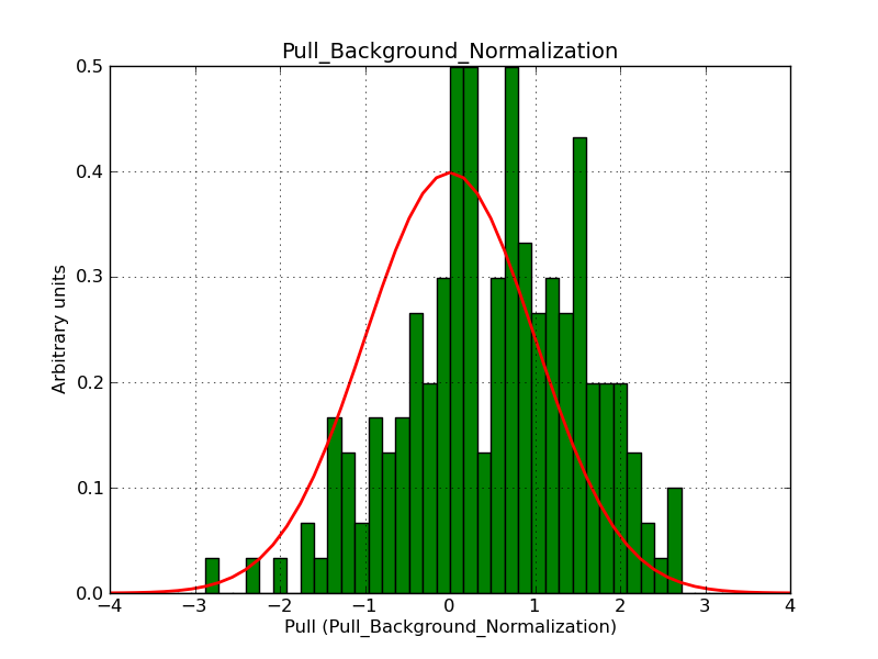
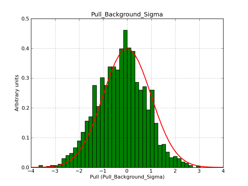
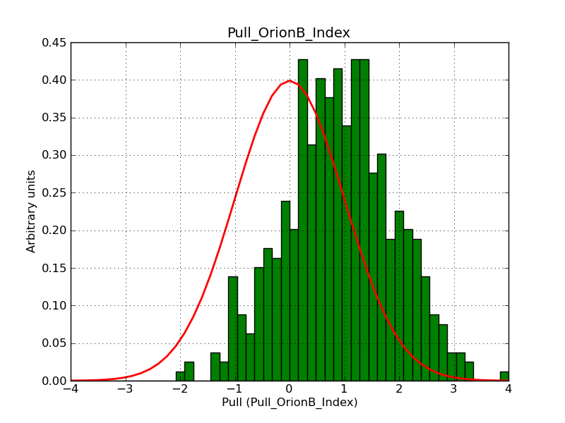
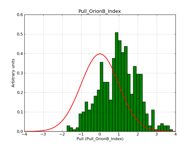
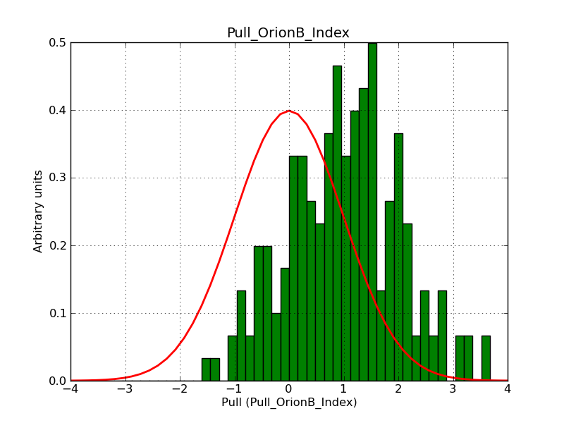
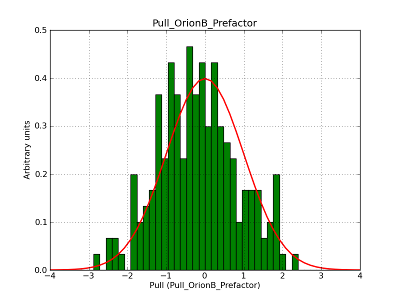
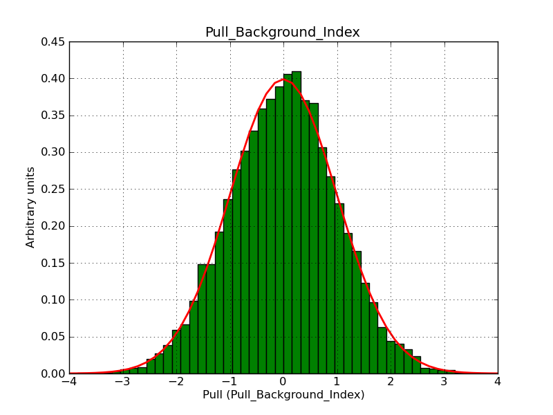
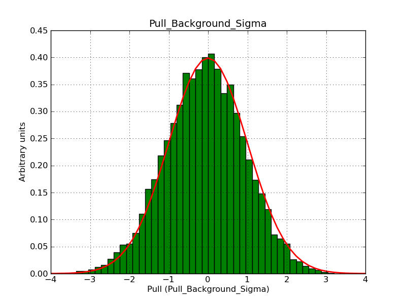
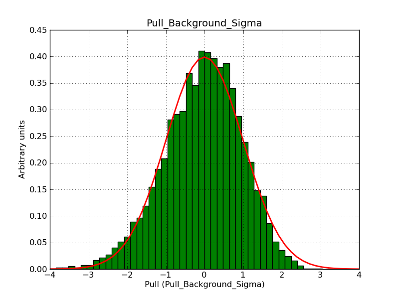
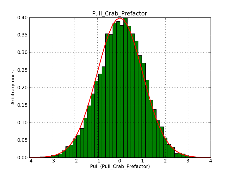
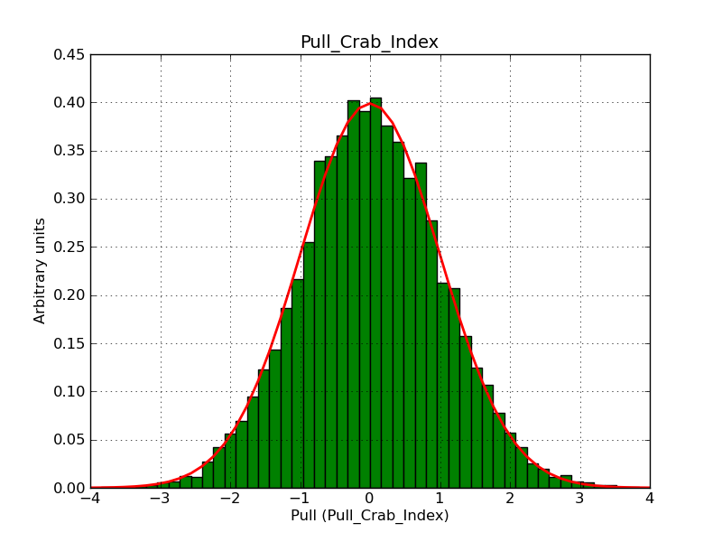
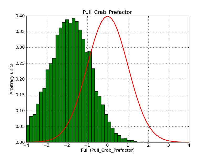
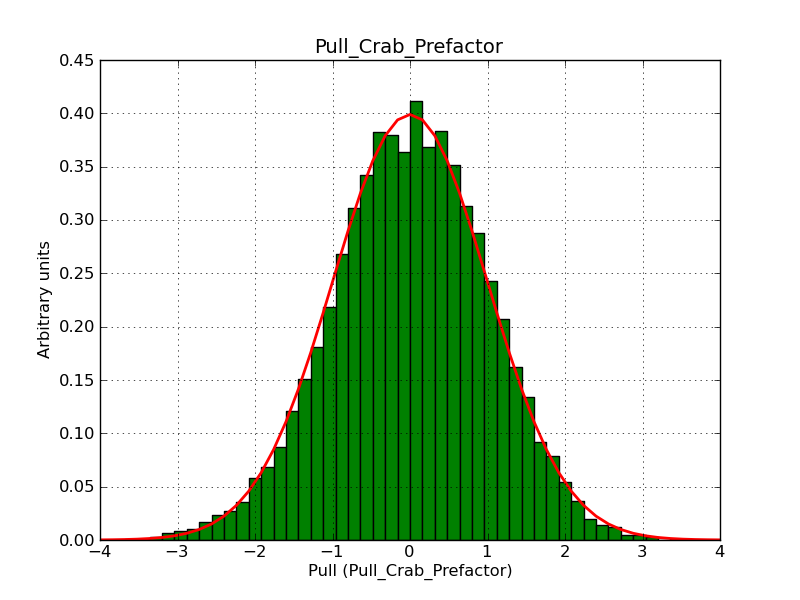
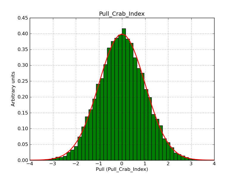
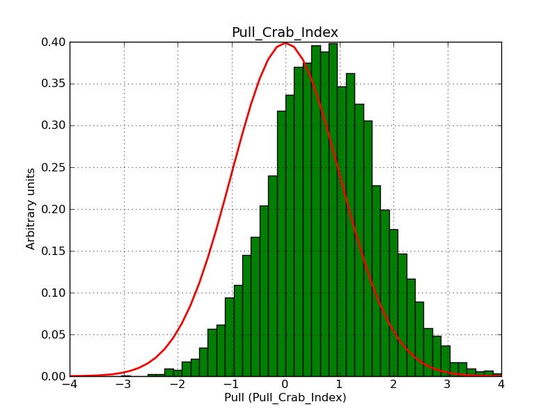
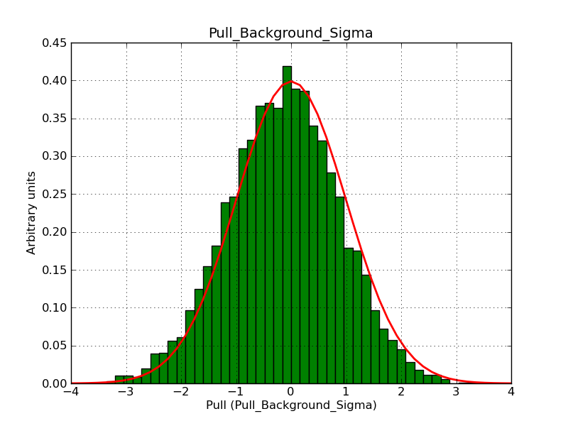
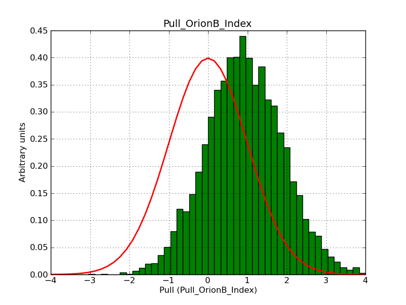
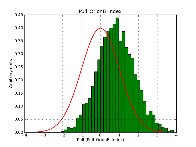
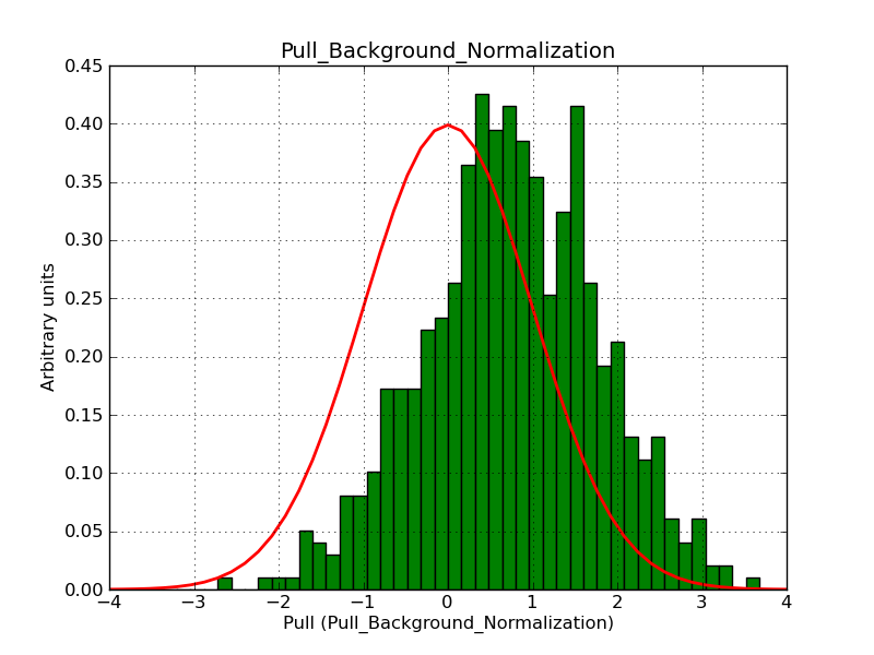
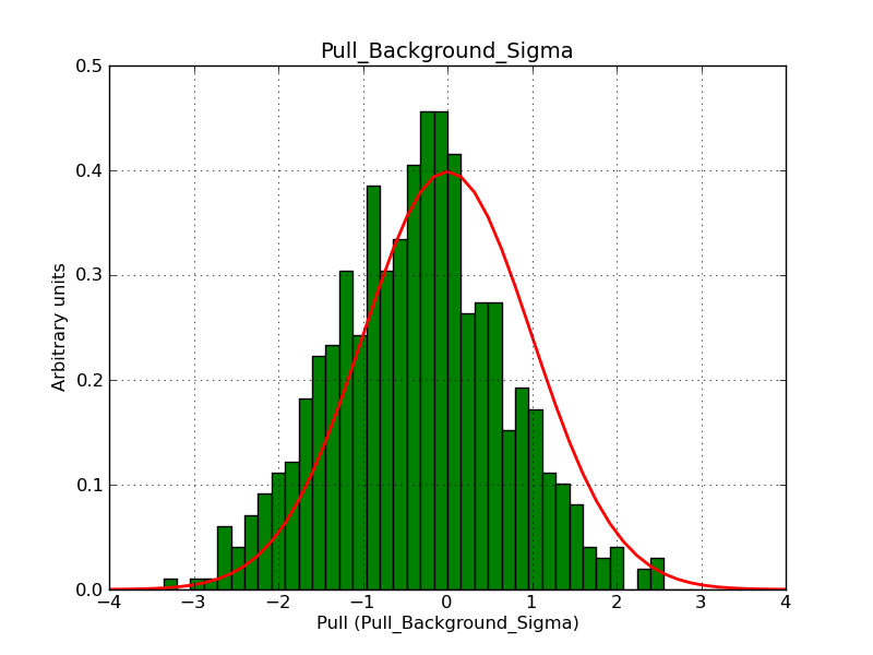
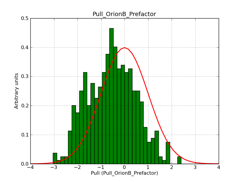
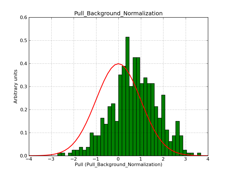
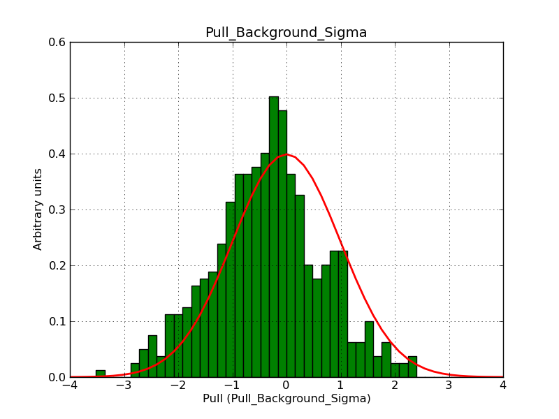
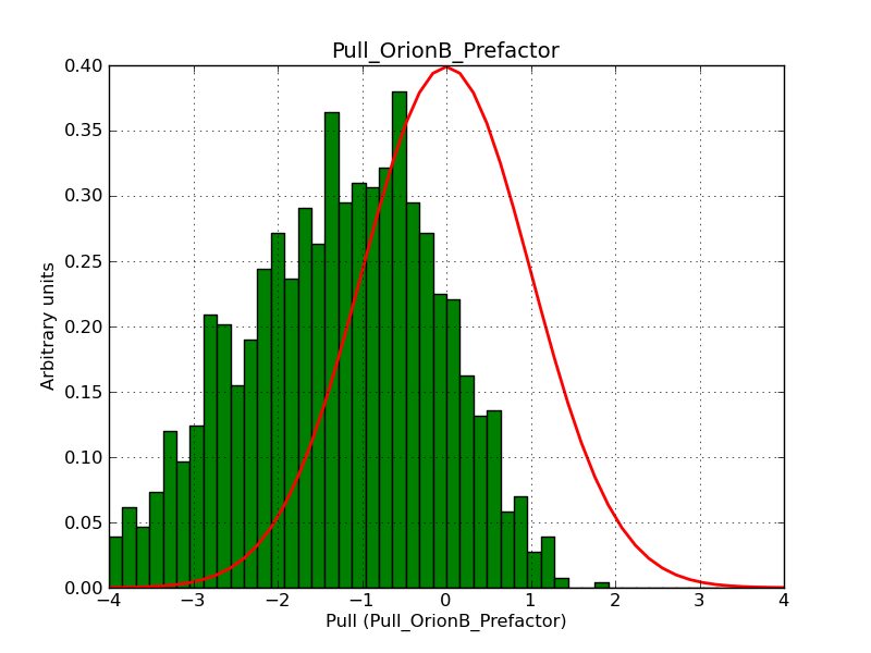
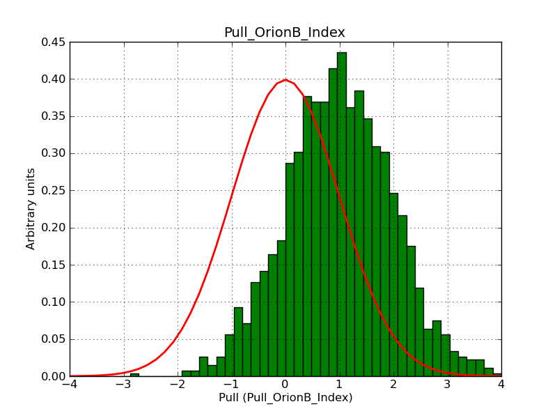
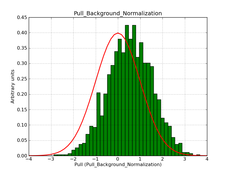
Preliminary pull distributions for the 4 free model parameters are shown below (a deadtime fraction of 5% has been assumed). The rows correspond to ROIs of 5° (first), 4° (second) and 3° (third). The last row is for a ROI of 5° with a pivot energy of 1 GeV.
 |
 |
 |
 |
 |
 |
 |
 |
 |
 |
 |
 |
 |
 |
 |
 |
Recurrence
No recurrence.
Related issues
History
#1
 Updated by Knödlseder Jürgen over 10 years ago
- File OrionB_Index_rad50_000802.png added
- File OrionB_Index_rad50_TeV_000802.png added
- File OrionB_Prefactor_rad30_TeV_000802.png added
- File OrionB_Prefactor_rad40_TeV_000802.png added
- File OrionB_Prefactor_rad50_000802.png added
- File OrionB_Prefactor_rad50_TeV_000802.png added
#2
 Updated by Martin Pierrick over 10 years ago
- File TSdistrib_smallfov.png added
- File TSdistrib_largefov.png added
- File Bgd-norm_largefov.png added
- File Bgd-norm_smallfov.png added
I did some tests with the following setup:
- The map provided by Akira as source with flux density 2e-18 ph/cm2/s/MeV at 1TeV and 2.7 as power-law index
- Background model with spatial part described by gaussian profile and spectral part by power law
- 100h observing time done in a single pointing
- Unbinned analysis from 500GeV-50TeV
- 50 trials
Results are OK and the spectral parameters are recovered by the fit. Typically, for 100h:
Mean/deviation of model 1 normalisation: 2.004213e-18 (6.165790e-20)
Mean/deviation of model 1 index: -2.708908 (0.054403)
... and for 50h:
Mean/deviation of model 1 normalisation: 1.956537e-18 (7.697961e-20)
Mean/deviation of model 1 index: -2.719990 (0.052099)
Distributions look good (but no formal pull distributions).
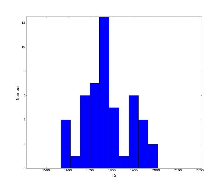
TS is of the order of 1700-1900 in the case of 100h, so very clear detection (assuming the true intensity distribution).
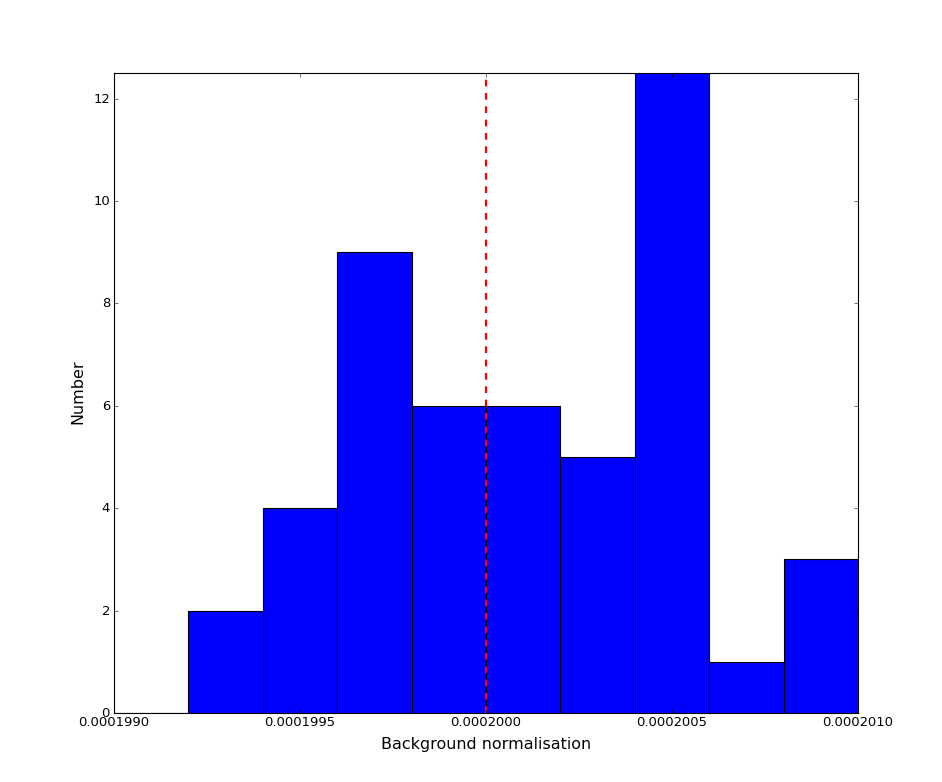
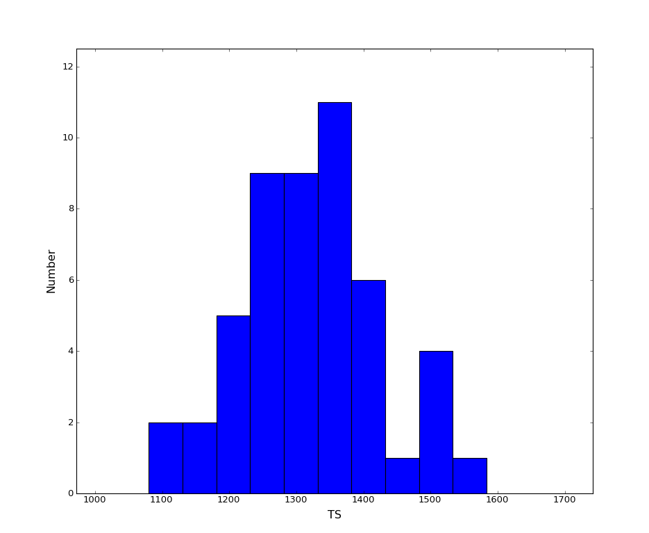
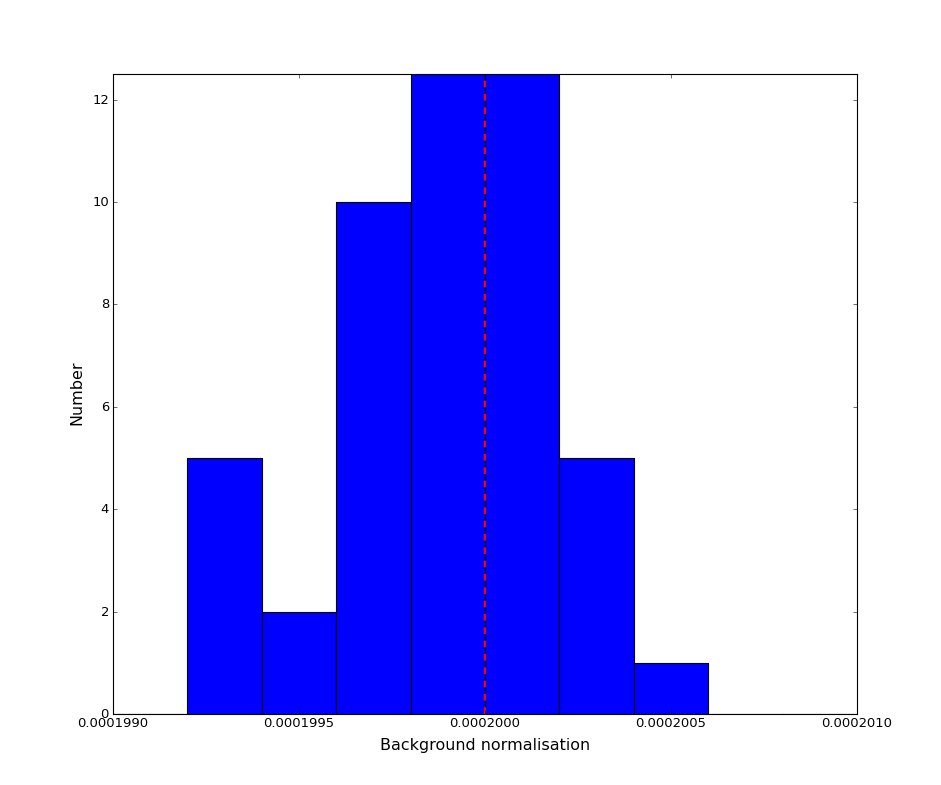
I tested the effect of the field-of-view size, which may affect the detection if it has a size ~ the size of the source. Moving from a size ~3deg to ~2deg (in radius), the TS drops to 1300-1400. In the same time, the background normalization distribution flattens and seems to extend more to higher values, which is expected if the background absorbs some of the source flux. See attached files. Note that the TS impact may also come from the null hypothesis.
Below plots for the small FOV (left) and the large FOV (right).
 |
 |
 |
 |
#3
 Updated by Knödlseder Jürgen over 10 years ago
- Status changed from New to In Progress
- Assigned To set to Knödlseder Jürgen
- Priority changed from Normal to High
- Target version set to 3rd coding sprint
- % Done changed from 0 to 60
#4
 Updated by Knödlseder Jürgen over 10 years ago
- Target version changed from 3rd coding sprint to 1.0.0
#5
 Updated by Knödlseder Jürgen about 10 years ago
- File gauss02_map_rad5_prefactor.png added
- File gauss02_map_rad5_index.png added
- File gauss02_map_rad5_bgd_prefactor.png added
- File gauss02_map_rad5_bgd_index.png added
- File gauss02_map_rad5_bgd_sigma.png added
- File gauss02_mapsmall_rad5_prefactor.png added
- File gauss02_mapsmall_rad5_index.png added
- File gauss02_mapsmall_rad5_bgd_prefactor.png added
- File gauss02_mapsmall_rad5_bgd_index.png added
- File gauss02_mapsmall_rad5_bgd_sigma.png added
I did some reinvestigation of this problem.
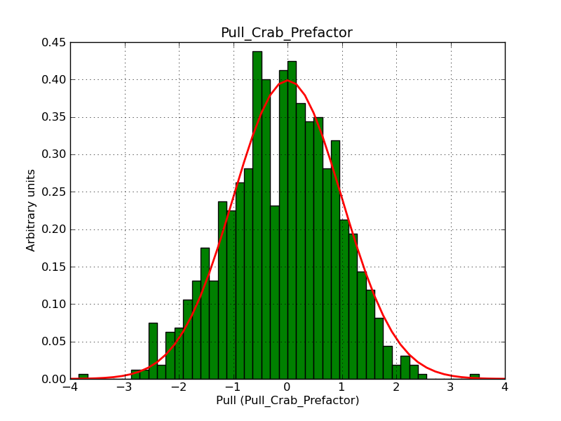
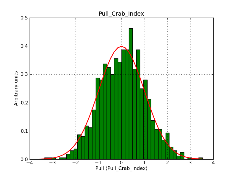
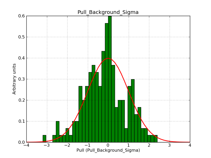
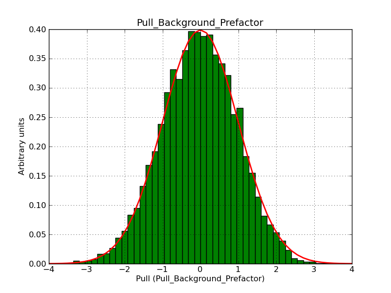
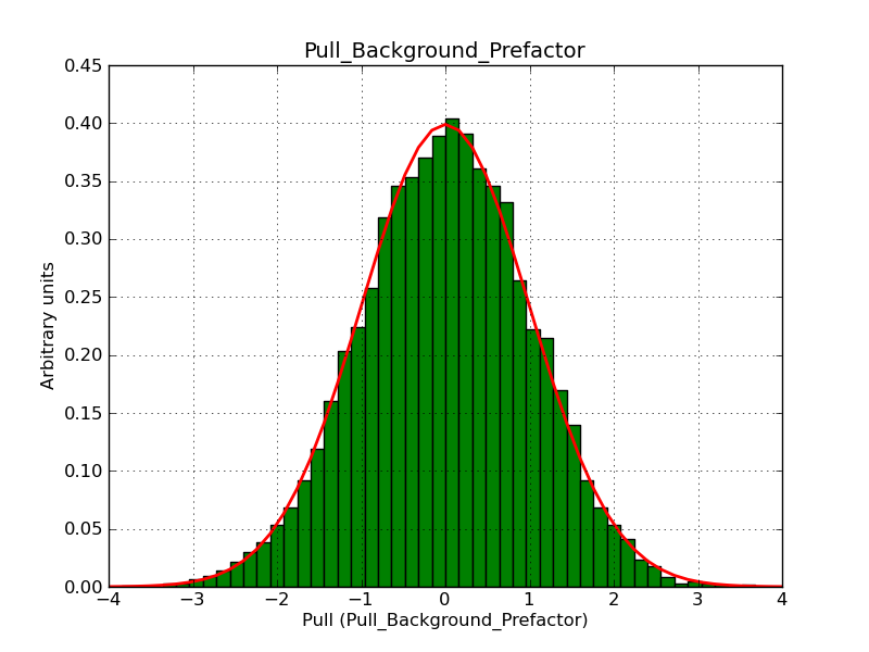
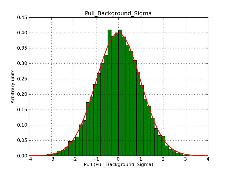
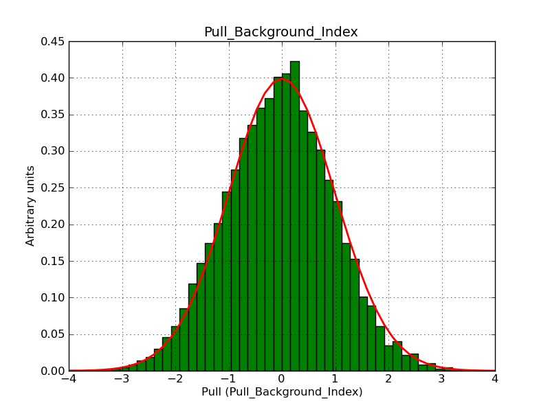
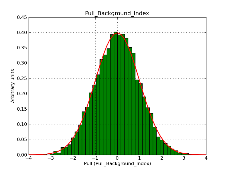
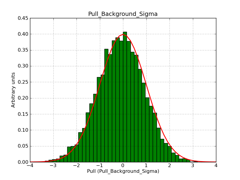
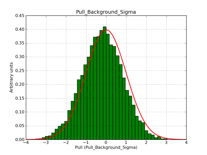
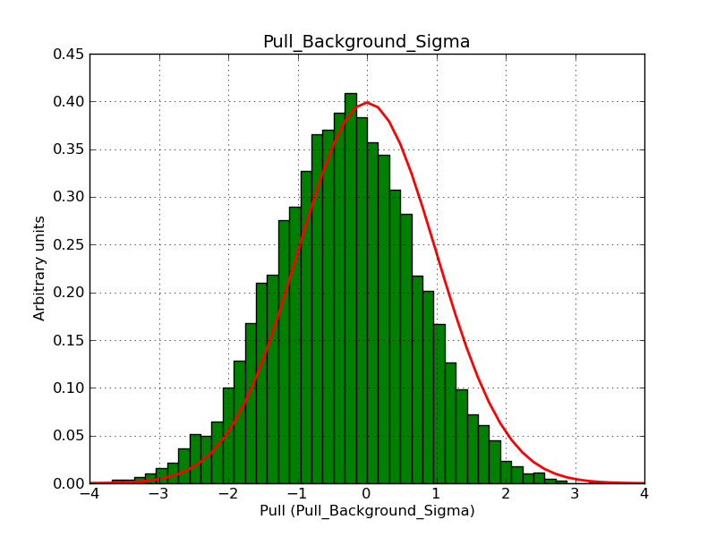
The model I used throughout is a Gaussian model with a sigma of 0.2 deg centred on the position of the Crab nebula and with a Crab nebula power law. I did some pull distributions using the Gaussian radial model and compared the results to the pull distributions obtained from a diffuse map that was computed from the Gaussian model. Ideally, both methods should provide identical results. Pull distributions were done for a dead time correction factor of 0.95, a duration of 1800 seconds, and for 10000 samples.
Below the results for the Gaussian radial model.
| Model | Prefactor | Index | Bgd. prefactor | Bgd. index | Bgd. sigma |
| ROI=5 deg |  |
 |
 |
 |
 |
| ROI=7 deg |
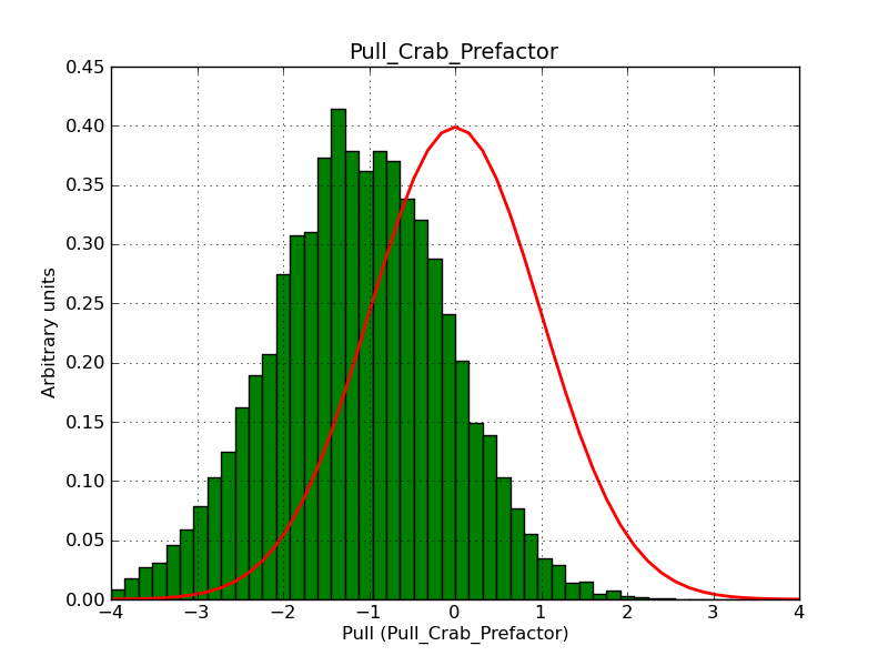
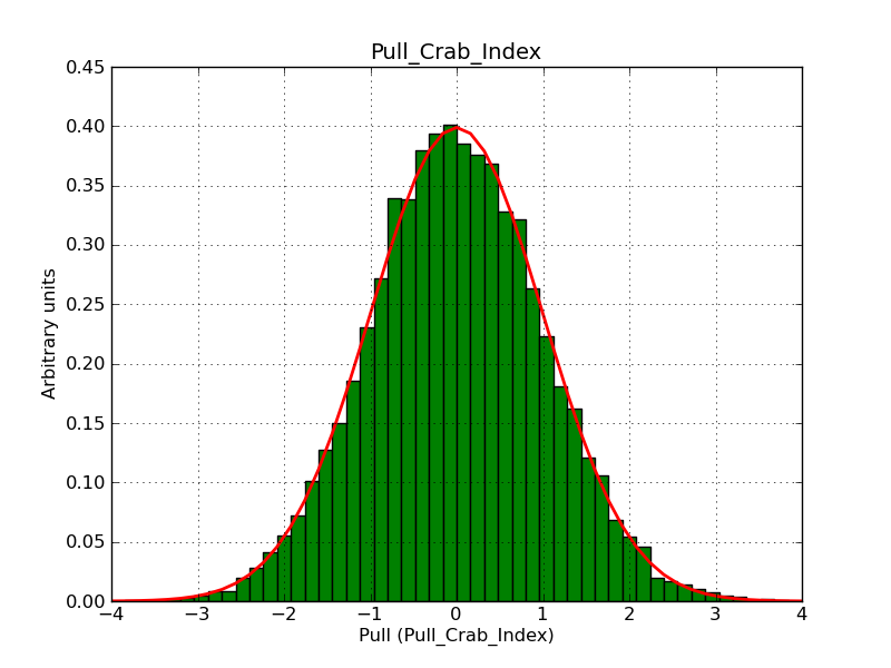
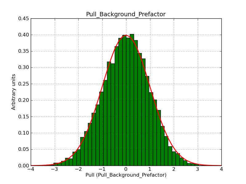
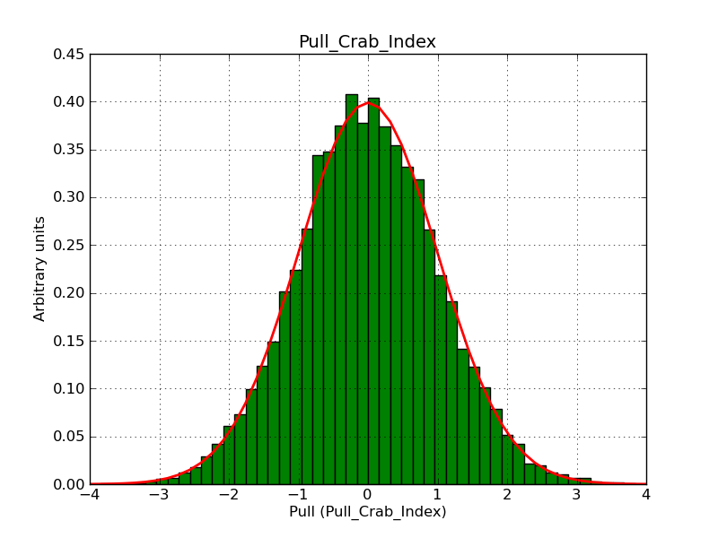
And here the results for the diffuse model. There is an obvious dependency on size of the ROI considered and size of the diffuse map (tiny is a 50x50 pixels map, small a 100x100 pixels map, large a 1000x1000 pixels map, all with a bin size of 0.01 degrees; all other runs were done with a 300x300 pixels map and a bin size of 0.01 degrees).
| Model | Crab Prefactor | Crab Index | Bgd. prefactor | Bgd. index | Bgd. sigma |
| ROI=2 deg | 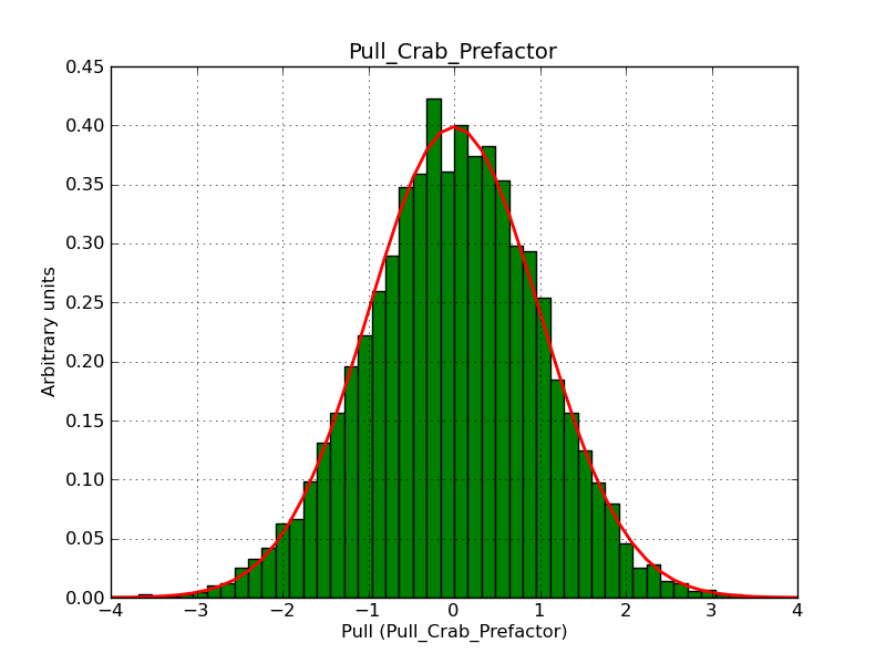 |
 |
 |
 |
 |
| ROI=3 deg |  |
 |
 |
 |
 |
| ROI=4 deg | 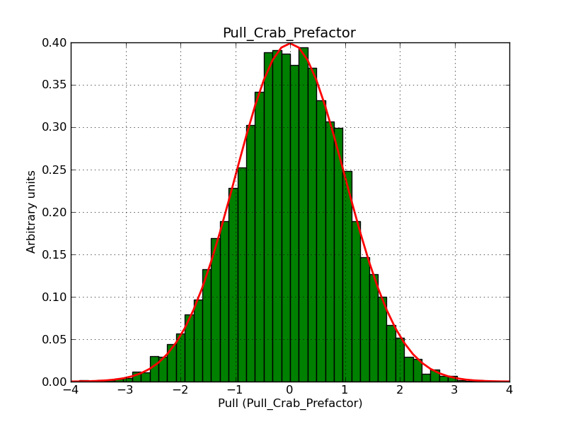 |
 |
 |
 |
 |
| ROI=5 deg |  |
 |
 |
 |
 |
| ROI=5 deg, tiny map | 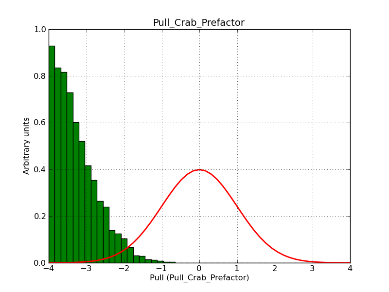 |
 |
 |
 |
 |
| ROI=5 deg, small map |  |
 |
 |
 |
 |
| ROI=5 deg, large map | 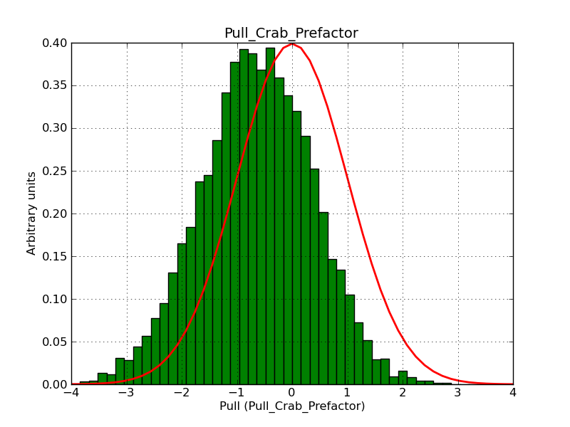 |
 |
 |
 |
 |
| ROI=6 deg |  |
 |
 |
 |
 |
| ROI=7 deg | 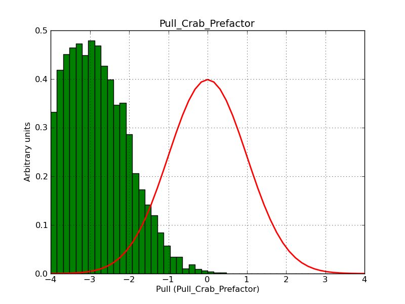 |
 |
 |
 |
 |
#6
 Updated by Knödlseder Jürgen about 10 years ago
- File gauss02_maplarge_rad5_prefactor.png added
- File gauss02_maplarge_rad5_index.png added
- File gauss02_maplarge_rad5_bgd_prefactor.png added
- File gauss02_maplarge_rad5_bgd_index.png added
- File gauss02_maplarge_rad5_bgd_sigma.png added
- % Done changed from 60 to 70
#7
 Updated by Knödlseder Jürgen about 10 years ago
- File gauss02_map_rad2_prefactor.png added
- File gauss02_map_rad2_index.png added
- File gauss02_map_rad2_bgd_prefactor.png added
- File gauss02_map_rad2_bgd_index.png added
- File gauss02_map_rad2_bgd_sigma.png added
- File gauss02_map_rad3_prefactor.png added
- File gauss02_map_rad3_index.png added
- File gauss02_map_rad3_bgd_prefactor.png added
- File gauss02_map_rad3_bgd_index.png added
- File gauss02_map_rad3_bgd_sigma.png added
#8
 Updated by Knödlseder Jürgen about 10 years ago
- File gauss02_map_rad4_prefactor.png added
- File gauss02_map_rad4_index.png added
- File gauss02_map_rad4_bgd_prefactor.png added
- File gauss02_map_rad4_bgd_index.png added
- File gauss02_map_rad4_bgd_sigma.png added
- File gauss02_map_rad6_prefactor.png added
- File gauss02_map_rad6_index.png added
- File gauss02_map_rad6_bgd_prefactor.png added
- File gauss02_map_rad6_bgd_index.png added
- File gauss02_map_rad6_bgd_sigma.png added
#9
 Updated by Knödlseder Jürgen about 10 years ago
- File gauss02_map_rad7_prefactor.png added
- File gauss02_map_rad7_index.png added
- File gauss02_map_rad7_bgd_prefactor.png added
- File gauss02_map_rad7_bgd_index.png added
- File gauss02_map_rad7_bgd_sigma.png added
#10
 Updated by Knödlseder Jürgen about 10 years ago
- File gauss02_rad5_prefactor.png added
- File gauss02_rad5_index.png added
- File gauss02_rad5_bgd_prefactor.png added
- File gauss02_rad5_bgd_index.png added
- File gauss02_rad5_bgd_sigma.png added
- File gauss02_maptiny_rad5_prefactor.png added
- File gauss02_maptiny_rad5_index.png added
- File gauss02_maptiny_rad5_bgd_prefactor.png added
- File gauss02_maptiny_rad5_bgd_index.png added
- File gauss02_maptiny_rad5_bgd_sigma.png added
#11
 Updated by Knödlseder Jürgen almost 10 years ago
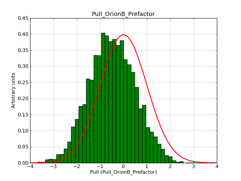
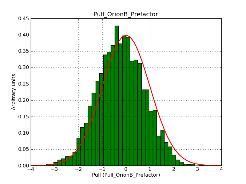
For the Orion simulation, only iter=9 seems to give satisfactory results. This however has an impact on computation speed. Here the value for iter=9:
 Unbinned instrument response computation (Npred):
 =================================================
  Estimated number of counts : 366.351 events
  Estimated - expected ......: -1.649 events (-0.4%)
  Elapsed time ..............: 14.324 sec
and here the result for the old value (
iter=6):Unbinned instrument response computation (Npred): ================================================= Estimated number of counts : 366.198 events Estimated - expected ......: -1.802 events (-0.5%) Elapsed time ..............: 0.300 sec
The code is about a factor of 50 slower.
#12
 Updated by Knödlseder Jürgen almost 10 years ago
- File pull_index_iter8.png added
- File pull_index_iter9.png added
- File pull_prefactor_iter8.png added
- File pull_prefactor_iter9.png added
Here the prefactor (left) and index (right) pull distributions for iter=8 (top) and iter=9 (bottom). While the prefactor is becoming better, the index pull distribution does not really evolve with number of iterations.
 |
 |
 |
 |
#13
 Updated by Knödlseder Jürgen over 9 years ago
- File rad5_tiny_index.png added
- File rad5_tiny_prefactor.png added
- File rad6_index.png added
- File rad6_prefactor.png added
- File rad7_index.png added
- File rad7_prefactor.png added
After restricting the pre-computations of the diffuse map to the simulation cone (see #1548) the biases in the prefactor and index that have been previously observed in the simulations of the Gaussian maps have disappeared. Below a few pull distributions for configurations that have shown problems before:
| r=5° (tiny map) |  |
 |
| r=6° |  |
 |
| r=7° | 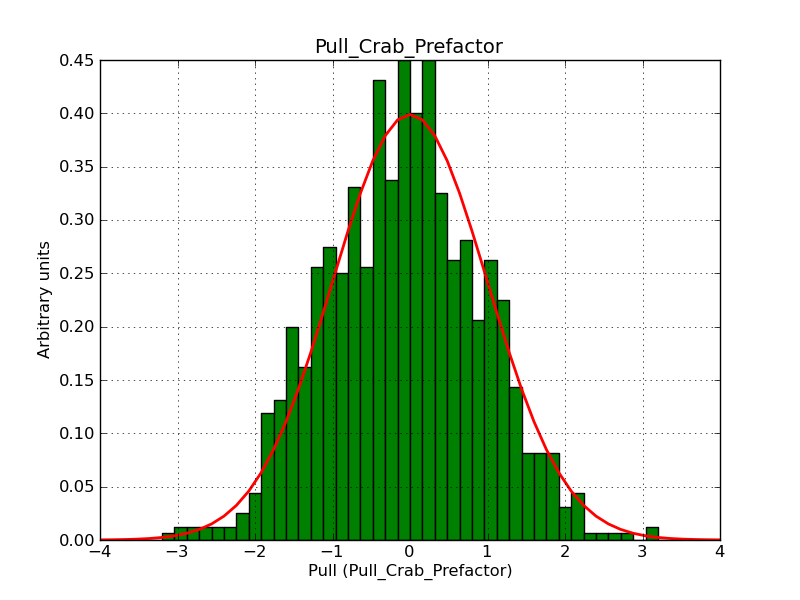 |
 |
#14
 Updated by Knödlseder Jürgen over 9 years ago
I now investigated how a change in the IRF integration precision (irf_diffuse method) impacts the resulting fits.
I examined the change when changing the IRF integration precision from 5 to 6. The checks have been done for the Cen A model and the Orion model. The following tables show the resulting spectral parameters for 3 trial runs:
Cen A:| Prefactor (5) | Index (5) | Prefactor (6) | Index (6) | Prefactor (change) | Index (change) |
| 5.69603e-16 | -2.49645 | 5.69549e-16 | -2.49641 | -0.009 % | -0.002 % |
| 5.5829e-16 | -2.49453 | 5.58157e-16 | -2.49444 | -0.024 % | -0.004 % |
| 5.42031e-16 | -2.44059 | 5.42057e-16 | -2.44059 | +0.005 % | 0.0 % |
| Prefactor (5) | Index (5) | Prefactor (6) | Index (6) | Prefactor (change) | Index (change) |
| 1.9074e-18 | -2.6532 | 1.90952e-18 | -2.6538 | +0.11 % | +0.023 % |
| 1.8521e-18 | -2.66186 | 1.85423e-18 | -2.66246 | +0.11 % | +0.023 % |
| 1.91605e-18 | -2.67305 | 1.91832e-18 | -2.6737 | +0.12 % | +0.024 % |
The change in the spectral parameters is negligible (well below 1%), hence a precision of 5 is sufficient for the irf_diffuse method.
#15
 Updated by Knödlseder Jürgen over 9 years ago
Now the same for the nroi_diffuse method. I first reduced the precision from 9 to 8 (first 2 tables) and then increased the precision from 9 to 10.
| Prefactor (9) | Index (9) | Prefactor (8) | Index (8) | Prefactor (change) | Index (change) |
| 5.69603e-16 | -2.49645 | 5.67596e-16 | -2.49572 | -0.35 % | -0.029 % |
| 5.5829e-16 | -2.49453 | 5.56217e-16 | -2.49373 | -0.37 % | -0.032 % |
| 5.42031e-16 | -2.44059 | 5.40025e-16 | -2.43973 | -0.37 % | -0.035 % |
| Prefactor (9) | Index (9) | Prefactor (8) | Index (8) | Prefactor (change) | Index (change) |
| 1.9074e-18 | -2.6532 | 1.89656e-18 | -2.65279 | -0.57 % | -0.015 % |
| 1.8521e-18 | -2.66186 | 1.84136e-18 | -2.6615 | -0.58 % | -0.014 % |
| 1.91605e-18 | -2.67305 | 1.90529e-18 | -2.67277 | -0.56 % | -0.010 % |
| Prefactor (9) | Index (9) | Prefactor (10) | Index (10) | Prefactor (change) | Index (change) |
| 5.69603e-16 | -2.49645 | 5.69123e-16 | -2.49609 | -0.084 % | -0.014 % |
| 5.5829e-16 | -2.49453 | 5.57794e-16 | -2.49415 | -0.089 % | -0.015 % |
| 5.42031e-16 | -2.44059 | 5.41557e-16 | -2.44021 | -0.088 % | -0.016 % |
| Prefactor (9) | Index (9) | Prefactor (10) | Index (10) | Prefactor (change) | Index (change) |
| 1.9074e-18 | -2.6532 | 1.90837e-18 | -2.6537 | +0.051 % | +0.019 % |
| 1.8521e-18 | -2.66186 | 1.85306e-18 | -2.66237 | +0.052 % | +0.019 % |
| 1.91605e-18 | -2.67305 | 1.91699e-18 | -2.67357 | +0.049 % | +0.019 % |
Reducing the precision to 8 could be acceptable as the changes are still smaller than 1%, but this may not be true for all possible sky maps. Having a precision of 9 seems to be on the save side. Increasing the precision to 10 is not necessary.
Hence a precision of 9 is adequate.
#16
 Updated by Knödlseder Jürgen over 9 years ago
- Status changed from In Progress to Closed
- % Done changed from 70 to 100
This issue can now be closed.
The remaining offset in the pull distribution can be explained by the precision of the GSkyMap::flux() method.


