Feature #753
Introduce GCTAPsfKing class
| Status: | Closed | Start date: | 02/14/2013 | |
|---|---|---|---|---|
| Priority: | Normal | Due date: | ||
| Assigned To: | % Done: | 100% | ||
| Category: | - | |||
| Target version: | 00-08-00 | |||
| Duration: |
Description
For model analysis in HESS the 68% containment radius of the PSF is computed by integrating over the actual shape. In fact, this shape differs significantly from a single Gaussian. One way to parameterise the PSF is a composition of three Gaussians with different widths, similar to GCTAPsf2D. The other way, which also has been done before, is to parameterise the PSF with a Student’s t-distribution. This function has only one parameter which can be calculated using the 68% containment radius.
Since the R68 of the PSF is the only parameter which is stored in model lookup tables, it would be nice to have a proper parameterisation of the PSF with only one parameter. My suggestion would be to include a class GCTAPsfStudentsT which inherits from GCTAPsfVector and just overwrites the functions like operator(), mc() and delta_max().
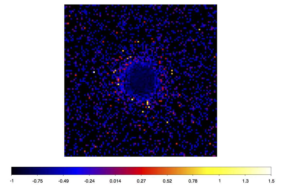
This class would also help to better compare results from gammalib with HESS-Analyses because the PSF would be modelled properly. Attached is a residual map (data-model)/model of the Crab Nebula using the a single Gaussian PSF. You can clearly see a ring-like excess originating from a bad parametrisation of the PSF. 
Recurrence
No recurrence.
History
#1
 Updated by Knödlseder Jürgen almost 12 years ago
I agree that we should implement this class. Good that the refactorisation of the CTA response is now finished, which allows easy addition of new Psf classes.
GCTAPsfVector is not really planned as a base class, so it’s probably better to clone this class to implement the Student’s T class. In the long run, GCTAPsfVector may eventually disappear, it is mainly there to digest existing response data. So better not use this class as a base class.
#2
 Updated by Deil Christoph almost 12 years ago
- File psf_models.html
 added
added - File psf_models.ipynb added
+1 to having this in gammalib.
Manuel, you are aware of the HESS internal note on the PSF and morphology fitting, right?
https://bitbucket.org/hess_software/hess_psf/downloads/HESS_PSF_Morphology_2013-02-07.pdf
https://bitbucket.org/hess_software/hess_psf/wiki/PSF_Models
(this is HESS internal because it contains confidential information)
I looked into the one-parameter Student T distribution Kora used in her thesis and found out that it is actually a special case of the two-parameter King profile that Fermi uses, and that the King profile is normalized to integrate to one, which is important for the PSF.
I think we should implement the King PSF (or make it usable for HESS if it is already there) and then the Student T will just be a special case.
See the attached IPython notebook that I used to learn some basic things about PSFs.
Here is the formula I implemented for KING a week ago (it looks different because it is the probability density in the theta square histogram that we usually fit):
http://www.mpi-hd.mpg.de/hfm/HESS/intern/Software/SASH-Docs/PSFInfo_8C_source.html
00614   else if( fitfunction == "TRIPLEEXP" ){
00615
00616     func =  new TF1( fname.c_str(),
00617              "[0]*(exp(-x/(2*[1]*[1]))+[2]*exp(-x/(2*[3]*[3]))+[4]*exp(-x/(2*[5]*[5])))",
00618              0.000, 0.05 );
00619
00620     double m = psf->GetMaximum();
00621     func->SetParameters( m, 0.01, 0.1, 0.1, 0.1, 0.2 );
00622     func->SetParLimits(0,0.001,10000.);
00623     func->SetParLimits(1,0.0,1.0);
00624     func->SetParLimits(2,0.001,10000.);
00625     func->SetParLimits(3,0.0,1.0);
00626     func->SetParLimits(4,0.001,10000.);
00627     func->SetParLimits(5,0.0,1.0);
00628     func->SetParNames("scale", "#sigma_{1}", "A_{2}", "#sigma_{2}", "A_{3}", "#sigma_{3}");
00629   }
00630   else if( fitfunction == "KING" ){
00631
00632     func =  new TF1( fname.c_str(),
00633              "[0] / (2 * [1] * [1]) * (1 - 1 / [2]) * pow(1 + 1 / (2 * [2]) * x  / ([1] * [1]), -[2])",
00634              0.000, 0.05 );
00635
00636     func->SetParNames("scale", "sigma", "gamma");
00637     func->SetParameter("scale", 1);
00638     func->SetParLimits(0, 0.1, 10.);
00639     func->SetParameter("sigma", 0.05);
00640     func->SetParLimits(1, 0.0, 1.0);
00641     func->SetParameter("gamma", 1.5);
00642     func->SetParLimits(2, 1, 10.);
00643   }
#3
 Updated by Deil Christoph almost 12 years ago
- File king_profile_description.png added
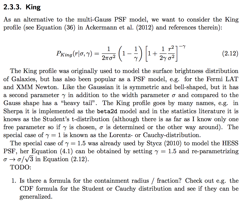
Attached find a short description of the King profile from the internal note.
Manuel and Jürgen: do you know if there are analytical formulae for containment fraction (for a given radius) and containment radius (for a given fraction)
for the triple-Gauss and King profile? That would be useful to have for me. (and I guess also for gammalib?)
#4
 Updated by Knödlseder Jürgen almost 12 years ago
The King function exists indeed for Fermi but not for CTA. If the Student’s T is just a special case of the King function, we better go for implementing the King function.
Concerning the analytical formulae: I guess the answer is no for a Gaussian, which needs numerical integration. For the King function you may check GLATPsfV3::base_int:
/***********************************************************************//**
 * @brief Return approximation of point spread base function integral
 *
 * @param[in] u Function argument.
 * @param[in] gamma Index.
 *
 * The version 3 PSF base function integral is approximated by
 * \f[1 - \left(1 + \frac{u}{\Gamma} \right)^{1-\Gamma}\f]
 * which is valid for small angles \f$u\f$. For larger angles a numerical
 * integration of the base function has to be performed.
 *
 * @todo Verify that 1+u/gamma is not negative
 ***************************************************************************/
double GLATPsfV3::base_int(const double& u, const double& gamma)
{
    // Compute integral of base function
    double integral = 1.0 - std::pow(1.0 + u/gamma, 1.0 - gamma);

    // Return integral
    return integral;
}
By the way, here a link to information about the Fermi PSF: http://fermi.gsfc.nasa.gov/ssc/data/analysis/documentation/Cicerone/Cicerone_LAT_IRFs/IRF_PSF.html
#5
 Updated by Deil Christoph almost 12 years ago
- File gauss_containment.png added
For a single Gauss there are simple analytical formulae for containment fraction and radius (see attached screenshot gauss_containment.png).
No numerical integration needed to compute those.
For the multi-Gauss I didn’t have time to think about it yet, if one of you figures it out (or knows of a reason why there shouldn’t be a formula), please let me know.
#6
 Updated by Knödlseder Jürgen almost 12 years ago
You’re absolutely right, I forgot that integration works analytically in 2D 
As the 3 Gaussians is just a linear combination, it should also work analytically for the 3 Gaussian PSF ...
#7
 Updated by Mayer Michael almost 12 years ago
- Subject changed from Introduce GCTAPsfStudentsT class to Introduce GCTAPsfKing class
- Description updated (diff)
First, Christoph I think you mean Michael instead of Manuel, right? 
Of course I knew about the PSF internal note... In fact, it was Kora’s suggestion to implement the Student’s T function when she saw my residuals. I absolutely agree, that since this function is just a special case of the King Profile, we should implement this instead. Hence, I changed the topic of this thread.
The King Profile can be integrated analytically. But I am still struggling to derive the parameter sigma for a given R68.
In my opinion, the following equation has to be solved to find sigma:
In the HESS lookup tables R68 is calculated without parameterising the PSF. It is done by integrating over Monte Carlo Theta2-distributions for point sources (as far as I know). Therefore, we need to calculate the corresponding sigma to a given R68 (and gamma). So far, I didn’t find an analytical way to do this.
I already started to create the files GCTAKing.hpp and .cpp. I would use GCTAPsf instead of GCTAPsfVector as a base class, if that is fine with you.
#8
 Updated by Knödlseder Jürgen almost 12 years ago
Sounds great.
I created a new Wiki entry for the PSF handling in CTA: GCTAPsf.
Can you add the relevant formulae (in particular the one for the King function) to this Wiki? By seeing the formula, maybe someone can provide some hint on how to integrate the profile.
#9
 Updated by Knödlseder Jürgen almost 12 years ago
- Assigned To set to Mayer Michael
#10
 Updated by Knödlseder Jürgen almost 12 years ago
- Target version set to 00-08-00
#11
 Updated by Deil Christoph almost 12 years ago
- R(sigma, gamma, F)
- F(sigma, gamma, R)
- sigma(gamma, R, F)
My approach would be to try with Mathematica, starting with simple special cases for gamma.
I don’t remember if I did try this already, if you can’t figure it out I can give it a shot at the weekend.
Note that there might not be an analytical solution for these functions, but the wiki page with the formulae and at least stating what we already tried to derive them is a very good idea.
#12
 Updated by Mayer Michael almost 12 years ago
- File sig_r68.png added
- File slope_gamma.png added
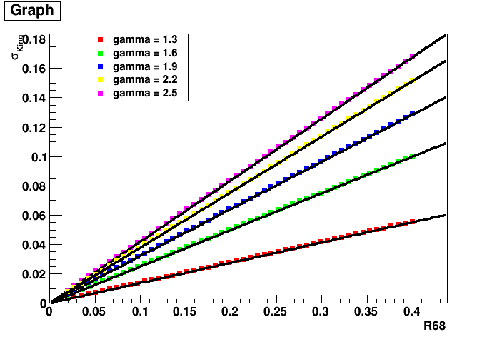
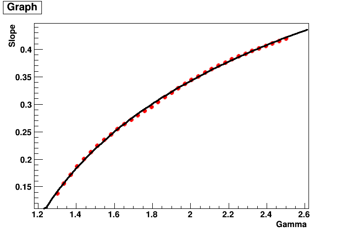
Yes, I want to find a formula for sigma(gamma,R68,F) with F being 0.68. I did some simulations for various parameters of gamma, sigma and r68, maybe to find an easy relation between those. In fact, for a fixed gamma, the relation between sigma and r68 couldn’t be easier: It is just a straight line from the origin. The slope of this line again depends on gamma (see plots). The relation between gamma and the slope is a bit more complex but also well fit by a logarithmic function. I found the following relation between the slope S and gamma:
Hence, we could easily parameterise sigma(gamma,R68) at least for the case of F = 0.68 and gamma between 1.2 and 2.5 (I think this might also be the range of gamma in the Fermi PSF?).
I am not sure wether we also need this also dependent on the containment fraction F since R68 is the most commonly used value (maybe we could also do for R95?). By the way: Is F=0.68 exactly, or is the real value more like 0.6827?
#13
 Updated by Knödlseder Jürgen almost 12 years ago
- File gammalib_maths.pdf added
- File slope_vs_gamma.png added
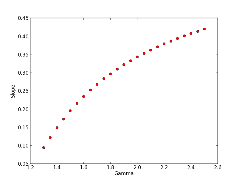
Attached a document that provides the analytic formulae: gammalib_maths.pdf.
The linearity between sigma and r68 is seen in Eq. (9) of section 2.1. The slope is given by Eq. (8), which differs from your equation. Below the graphical representation of Eq. (8) to compare with your slope plot. For large gammas the plot seems to fit yours, but for small gammas I find smaller values than you do. Could this be a numerical problem in your estimate, as for small gammas the r68 becomes very large?
#14
 Updated by Knödlseder Jürgen almost 12 years ago
- File gammalib_maths.pdf added
#15
 Updated by Knödlseder Jürgen almost 12 years ago
- File deleted (
gammalib_maths.pdf)
#16
 Updated by Knödlseder Jürgen almost 12 years ago
- File king.py
 added
added
For the record, here is a small Python script that checks the analytical formulae: king.py
#17
 Updated by Knödlseder Jürgen almost 12 years ago
- Target version changed from 00-08-00 to HESS sprint #1
#18
 Updated by Mayer Michael almost 12 years ago
Thanks a lot for that input! I definitely should have read that document before . I just did a different substitution to solve the integral and hence the equation became a mess. I am sure, that the deviation for small gammas was a computational problem of my “quick & dirty” way to find a solution:). I will incorporate your solution in the code, thanks.
#19
 Updated by Knödlseder Jürgen over 11 years ago
- Target version changed from HESS sprint #1 to 00-08-00
#20
 Updated by Knödlseder Jürgen about 11 years ago
- Target version deleted (
00-08-00)
#21
 Updated by Mayer Michael about 11 years ago
This project is almost ready, In fact, the files were on my computer for the last months. However, the reader still needs to be written and also some thinking is required how to handle the new format. One would need an operator(double lnE,double det_x, double det_y, ...) to access the PSF, which probably also has to exist in the base class, too.
#22
 Updated by Knödlseder Jürgen about 11 years ago
Great. I can move it of course back into the 0.8.0 target.
#23
 Updated by Mayer Michael about 11 years ago
- % Done changed from 0 to 80
Just to give a short update: The code is working. I still have to test the mc()-method. If this was done successfully, I will push the branch into the repository. As input format, I followed a GCTAResponseTable using a GFitsTable as input.
#24
 Updated by Mayer Michael about 11 years ago
753-Introduce-GCTAPsfKing. There are still some things which need testing:
- the
mc()-Method has not been tested at all, so there will probably be errors in it. - the
delta_max()-Method requires some thinking because if we use e.g. 99% containment, the radius can be quite large due to the long tails of this function. If the return value of this function is too large, the computation will take forever. Preliminary, the value has been set fixed to 0.7 degrees, which should be sufficient for IACT analysis.
#25
 Updated by Mayer Michael about 11 years ago
- Status changed from New to Feedback
- % Done changed from 80 to 90
#26
 Updated by Knödlseder Jürgen about 11 years ago
I merged your branch in the integration branch and added a unit test. The King profile PSF is now in the irf_test.fits file under bcf/000002 directory. I modified GCTAResponse::load_psf so that the King profile PSF file is automatically detected. I also modified GCTAResponse::load so that a FITS file can be specified. Both functionalities are used in the unit test.
I added a compile option to GCTAPsfKing so that the fixed delta_max option can be enabled or disabled (for testing purposes). Furthermore, I added some code so that the integral under the fixed delta_max is always 1. Specifically, the operator() now returns 0 if delta>delta_max. And the normalization factor is changed in the update method so that the intergral is correct.
This basically means that the PSF is now truncated at 0.7 deg. We may discuss if this is reasonable or not. If the PSF has really a tail going beyond 0.7 deg, we would underestimate the flux with this new method. I introduced the normalization mainly because the unit test gave in fact integrals that differed substantially from 1. I was thus wondering whether the King parameters were indeed reasonable, or whether the statistical noise creates sometimes parameter sets that predict infinitely large tails. When inspecting the King profile parameters, I recognized that the parameter distribution was not very smooth.
#27
 Updated by Knödlseder Jürgen about 11 years ago
- File psf_100GeV.png added
- File psf_1TeV.png added
- File psf_10TeV.png added
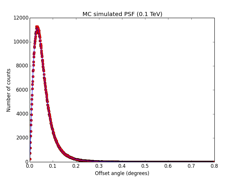
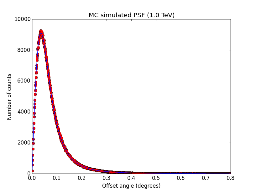
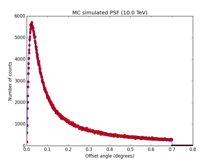
GCATPsfKing. I also added the truncation here. The script used to produce the plots is example_sim_psf.py in the cta/test folder. Looks all reasonable.
 |
 |
 |
#29
 Updated by Knödlseder Jürgen about 11 years ago
- Target version set to 00-08-00
#30
 Updated by Knödlseder Jürgen about 11 years ago
- Status changed from Feedback to Closed

