 Martin Pierrick
Updated almost 11 years ago by
The central GammaLib repo will be accessed using the https protocol, which makes use of SSL certificates. To disable certificate verification, we recommend to issue the command
$ git config --global http.sslverify "false"which disables certificate verification globally.
If you want to avoid typing your user name and password every time you make a push, you can create a file called .netrc under your root directory (i.e. ~/.netrc) with the following content:
machine cta-git.irap.omp.eu
  login <user>
  password <password>
(replace
<user> and <password> by your user name and password). Once the .netrc file in place, you may simply type$ git pushto push you code changes into the repository.
Note: There seems to be a problem with git version 1.7.11.3, which does not allow pushing a new branch in the central repository or even cloning an existing project (at least when used from a Mac with OS X 10.6.8). No password is requested when it should be, and the following message appears:
error: RPC failed; result=22, HTTP code = 401
fatal: The remote end hung up unexpectedly
Updated over 10 years ago by 
This section gives a summary of the workflow. Details are given for each of these steps in the following sections.
devel branch is the trunk.devel branch, and start a new feature branch from that.536-refactor-database-code.devel or any other branches into your feature branch while you are working.devel, consider Rebasing on devel.This way of working helps to keep work well organized, with readable history.
To clone the GammaLib source code, type
$ git clone https://user@cta-git.irap.omp.eu/gammalib
This will create a directory called ctools under the current working directory that will contain the ctools source code.
This will create a directory called gammalib under the current working directory that will contain the GammaLib source code. Here, user is your user name on the CTA collaborative platform at IRAP (the same you used to connect for reading this text). Executing this command will open a window that asks for a password (your password on the CTA collaborative platform at IRAP), and after confirming the password, your will get a clone of gammalib on your disk.
Note that the default branch from which you should start for software developments is the devel branch, and the git clone command normally automatically clone this branch from the central repository. Make sure that you will never use the master branch to start your software developments, as pushing to the master branch is not permitted. The master branch always contains the code of the last GammaLib release, and serves as seed for hotfixes. To know which branch you’re on, type
$ git status
devel, switch to the devel branch using$ git checkout devel
When you are ready to make some changes to the code, you should start a new branch. We call this new branch a feature branch.
The name of a feature branch should always start with the Redmine issue number, followed by a short informative name that reminds yourself and the rest of us what the changes in the branch are for. For example 735-add-ability-to-fly, or 123-bugfix. If you don’t find a Redmine issue for your feature, create one.
First make sure that you start from the devel branch by typing
$ git checkout develThen create a new feature branch using
$ git checkout -b 007-my-new-feature
Switched to a new branch '007-my-new-feature'
This creates and switches automatically to the branch
007-my-new-feature.
Now you’re ready to write some code and commit your changes. Suppose you edited the pyext/GFunction.i file. After editing, you can check the status by typing
$ git status
# On branch 007-my-new-feature
# Changes not staged for commit:
#   (use "git add <file>..." to update what will be committed)
#   (use "git checkout -- <file>..." to discard changes in working directory)
#
#    modified:   pyext/GFunction.i
#
no changes added to commit (use "git add" and/or "git commit -a")
Git signals here that you have to add and commit your change.
You’ll do this by typing
$ git add pyext/GFunction.i
$ git commit -am 'Remove GTools.hpp include.'
  [007-my-new-feature 065af59] Remove GTools.hpp include.
   1 files changed, 0 insertions(+), 1 deletions(-)
Continue with editing and commit all your changes.
To push your new feature branch into the IRAP git repository, type
$ git push origin 007-my-new-feature
  Password:
Counting objects: 7, done.
Delta compression using up to 48 threads.
Compressing objects: 100% (4/4), done.
Writing objects: 100% (4/4), 390 bytes, done.
Total 4 (delta 3), reused 0 (delta 0)
remote: To https://github.com/gammalib/gammalib.git
remote:    8139b97..07946a3  github/integration -> github/integration
remote:  * [new branch]      007-my-new-feature -> 007-my-new-feature
To https://jknodlseder@cta-git.irap.omp.eu/gammalib
 * [new branch]      007-my-new-feature -> 007-my-new-feature
This pushed your modifications into the repository. Note that this created a new branch in the repository.
Eventually, the devel branch has advanced while you developed the new feature. In this case, you should rebase your code before asking for merging. If you’re not sure what this means, better skip this step and leave it to the integration manager to work out how to deal with the diverged branches. If you feel however you want to help the manager with integration, rebase your branch using
$ git fetch origin
  Password:
$ git pull origin 007-my-new-feature
  Password:
  From https://cta-git.irap.omp.eu/gammalib
   * branch            007-my-new-feature -> FETCH_HEAD
  Already up-to-date.
$ git checkout 007-my-new-feature
  Already on '007-my-new-feature'
  Your branch and 'devel' have diverged,
  and have 1 and 1 different commit(s) each, respectively.
$ git branch tmp 007-my-new-feature
$ git rebase devel
  First, rewinding head to replay your work on top of it...
  Applying: Remove GTools.hpp include.
Here we created a backup of
007-my-new-feature into tmp for safety.
If your feature branch is already in the central repository and you rebase, you will have to force push the branch; a normal push would give an error. Use this command to force-push:
$ git pull origin 007-my-new-feature
  Password:
  From https://cta-git.irap.omp.eu/gammalib
   * branch            007-my-new-feature -> FETCH_HEAD
  Merge made by the 'recursive' strategy.
$ git push -f origin 007-my-new-feature
  Password:
  Counting objects: 5, done.
  Delta compression using up to 4 threads.
  Compressing objects: 100% (3/3), done.
  Writing objects: 100% (3/3), 492 bytes, done.
  Total 3 (delta 2), reused 0 (delta 0)
  remote: To https://github.com/gammalib/gammalib.git
  remote:    1f00150..20cf8c5  007-my-new-feature -> 007-my-new-feature
  remote:    35d6408..1f00150  github/007-my-new-feature -> github/007-my-new-feature
  To https://jknodlseder@cta-git.irap.omp.eu/gammalib
     1f00150..20cf8c5  007-my-new-feature -> 007-my-new-feature
Note that this will overwrite the branch in the central repository, i.e. this is one of the few ways you can actually lose commits with git.
Note: I don’t really understand why I need the git pull before the push, but without I get the following error message:
$ git push -f origin 007-my-new-feature
  Password:
  Counting objects: 11, done.
  Delta compression using up to 4 threads.
  Compressing objects: 100% (7/7), done.
  Writing objects: 100% (7/7), 1.44 KiB, done.
  Total 7 (delta 6), reused 0 (delta 0)
  remote: error: denying non-fast-forward refs/heads/007-my-new-feature (you should pull first)
When all looks good you can delete your backup branch using
$ git branch -D tmp
  Deleted branch tmp (was 1f00150).
When you are ready to ask for someone to review your code and consider a merge, change the status of the issue you’re working on to Pull Request:

In the notes field, describe the set of changes, and put some explanation of what you’ve done. Say if there is anything you’d like particular attention for - like a complicated change or some code you are not happy with.
If you don’t think your request is ready to be merged, just say so in your pull request message. This is still a good way of getting some preliminary code review.
Updated over 11 years ago by
As first step, a clone of the central GammaLib repository is needed:
$ git clone https://manager@cta-git.irap.omp.eu/gammalib
  Cloning into 'gammalib'...
  Password:
  remote: Counting objects: 22150, done.
  remote: Compressing objects: 100% (7596/7596), done.
  remote: Total 22150 (delta 17330), reused 18491 (delta 14497)
  Receiving objects: 100% (22150/22150), 80.12 MiB | 192 KiB/s, done.
  Resolving deltas: 100% (17330/17330), done.
where
manager is the user name of the integration manager.
If there are only a few commits, consider rebasing to upstream:
$ git checkout 007-my-new-feature
$ git fetch origin
$ git rebase origin/devel
If there are a longer series of related commits, consider a merge instead:
$ git checkout 007-my-new-feature
$ git merge --no-ff origin/devel
Note the
--no-ff above. This forces git to make a merge commit, rather than doing a fast-forward, so that these set of commits branch off devel then rejoin the main history with a merge, rather than appearing to have been made directly on top of devel.
Now, in either case, you should check that the history is sensible and you have the right commits:
$ git log --oneline --graph
$ git log -p origin/devel..
The first line above just shows the history in a compact way, with a text representation of the history graph. The second line shows the log of commits excluding those that can be reached from
devel (origin/devel), and including those that can be reached from current HEAD (implied with the .. at the end). So, it shows the commits unique to this branch compared to devel. The -p option shows the diff for these commits in patch form.
Now it’s time to merge the feature branch in the integration branch:
$ git checkout integration
  Branch integration set up to track remote branch integration from origin.
  Switched to a new branch 'integration'
$ git merge 007-my-new-feature
  Updating ccba491..623d38d
  Fast-forward
   .gitignore                |   20 ++++++++---
   pyext/GDerivative.i       |   77 +++++++++++++++++++++++++++++++++++++++++++++
   pyext/GFunction.i         |   46 +++++++++++++++++++++++++++
   pyext/gammalib/numerics.i |    2 +
   4 files changed, 139 insertions(+), 6 deletions(-)
   create mode 100644 pyext/GDerivative.i
   create mode 100644 pyext/GFunction.i
$ git push origin integration
  Password:
  Counting objects: 7, done.
  Delta compression using up to 4 threads.
  Compressing objects: 100% (4/4), done.
  Writing objects: 100% (4/4), 392 bytes, done.
  Total 4 (delta 3), reused 0 (delta 0)
  remote: To https://github.com/gammalib/gammalib.git
  remote:    ccba491..623d38d  integration -> integration
  remote:    065af59..8c6cc48  github/007-my-new-feature -> github/007-my-new-feature
  To https://jknodlseder@cta-git.irap.omp.eu/gammalib
     ccba491..623d38d  integration -> integration
The push will automatically launch the integration pipeline on Jenkins.
You should verify the all checks are passed with success.
Once the new feature is validated, merge the feature in the devel branch:
$ git checkout devel
  Switched to branch 'devel'
$ git merge integration
  Updating cb9b2fe..623d38d
  Fast-forward
   pyext/GFunction.i |    1 -
   1 files changed, 0 insertions(+), 1 deletions(-)
$ git push origin
  Total 0 (delta 0), reused 0 (delta 0)
  remote: To https://github.com/gammalib/gammalib.git
  remote:    cb9b2fe..623d38d  devel -> devel
  remote:    ccba491..623d38d  github/integration -> github/integration
  To https://jknodlseder@cta-git.irap.omp.eu/gammalib
     cb9b2fe..623d38d  devel -> devel
$ git checkout devel
  Already on 'devel'
$ git branch -D 007-my-new-feature
  Deleted branch 007-my-new-feature (was 816ac2c).
$ git push origin :007-my-new-feature
  Password:
  remote: To https://github.com/gammalib/gammalib.git
  remote:  - [deleted]         007-my-new-feature
  remote:    cb9b2fe..623d38d  github/devel -> github/devel
  To https://jknodlseder@cta-git.irap.omp.eu/gammalib
   - [deleted]         007-my-new-feature
Note the colon : before
007-my-new-feature. See also: http://github.com/guides/remove-a-remote-branch
Updated over 11 years ago by
The COMPTEL telescope aboard the CGRO satellite has been flown from 1991-2000, collecting an unprecedented set of data in the energy range from 750 keV up to 30 MeV. Some information about the COMPTEL telescope and access to the data can be found at the following link: http://heasarc.gsfc.nasa.gov/docs/cgro/comptel.
Although the COMPTEL database is very valuable, no software tools are publically available to exploit the COMPTEL data.
A description of the COMPTEL datasets can be found at http://wwwgro.unh.edu/comptel/comptel_datasets.html.
All COMPTEL data are available in FITS format. The following datasets are relevant for COMPTEL data analysis:Information about the processed data is available at http://wwwgro.unh.edu/comptel/compass/compass_users.html.
Here some further useful links concerning the data:The COMPTEL data were analysed using the COMPASS software that is not publically available.
Here some useful links:Updated almost 9 years ago by
The first step in a code release is to branch off the actual code in devel and merge it into the release branch. This is done for an authorized code manager using the following sequence of commands:
git checkout release
git merge devel
Before releasing the code, you have to modify a number of files to incorporate release information in the code distribution and to update the code version number. This may have been done before during the development. The command sequence for updating release information is:
git checkout release
nano configure.ac
  AC_INIT([gammalib], [0.10.0], [jurgen.knodlseder@irap.omp.eu], [gammalib])
nano gammalib.pc.in
  Version: 0.10.0
nano ChangeLog
  ... (update the change log) ...
nano NEWS
  ... (update the NEWS) ...
nano README
  ... (update the README) ...
nano doc/Doxyfile
  PROJECT_NUMBER         = 0.10.0
nano doc/source/conf.py
  # The short X.Y version.
  version = '0.10'
  # The full version, including alpha/beta/rc tags.
  release = '0.10.0'
git add *
git commit -m "Set release information for release X.Y.Z."
git push
The nano commands will open an editor (provided you have nano installed; otherwise use any other convenient editor). The lines following the nano command indicate which specific lines need to be changed. Changes in the files ChangeLog, NEWS and README need some more editing. Please take some time to write all important things done, as GammaLib users will later rely on this information for their work! ChangeLog and NEWS should have been updated while adding new features, but you probably need to adapt the version number and release date.
Use the release branch in the central repository to perform extended code testing. The code testing is done by the release pipeline in Jenkins. Make sure that this pipeline runs fully through before continuing. If errors occurred in the testing, correct them and run the pipeline again unit the pipeline ends with success. Don’t forget to push any changes into the repository.
In addition to the pipeline, apply the testall.sh script in the gammalib folder to check all test executables and scripts.
Use the script dev/release_gammalib.sh to build a tarball of the GammaLib release. This is usually done on the kepler.cesr.fr server. Should be moved into Jenkins.
Test that the tarball compiles and all checks run. Type
tar xvf ../gammalib-0.10.0.tar.gz
cd gammalib-0.10.0
./configure
make
make check
Should be moved into Jenkins.
TBW
Now you can merge the release branch into the master branch using the commands:
git checkout master
git merge release
Now you can tag the release using
git tag -a GammaLib-0.10.0 -m "GammaLib release 0.10.0"
git push --tags
We use here an annotated tag with a human readable tag message. Please use always the same format. In the above example, the GammaLib version X.Y.Z was 0.10.0.
Now we merge the master branch back in the devel branch to make sure that the devel branch incorporates all modifications that were made during the code release procedure.
git checkout devel
git merge release
git push
You now should being the devel branch ahead of the master branch. This means that the devel branch should have an additional commit with respect to the master branch. This is not mandatory, but it assures later that the master branch and the devel branch will never point to the same commit. In that way, git clone will always fetch the devel branch, which is the required default behavior.
To bring the devel branch ahead, execute following commands:
git checkout devel
nano AUTHORS
git add AUTHORS
git commit -m "Bring develop branch ahead of master branch after code release."
The nano AUTHORS step opens the file AUTHORS in an editor. Just add or remove a blank line to make a file modification.
Now you’re done!
Updated over 11 years ago by
This page summarizes the status of the GammaLib code.
Cppcheck is a static analysis tool for C/C++ code. Unlike C/C++ compilers and many other analysis tools it does not detect syntax errors in the code. Cppcheck primarily detects the types of bugs that the compilers normally do not detect. The goal is to detect only real errors in the code (i.e. have zero false positives).
In the frame below you find the latest Cppcheck result for GammaLib.
In the frame below you find the latest coverage result for GammaLib.
SLOCCount is a set of tools for counting physical Source Lines of Code (SLOC) in a large number of languages of a potentially large set of programs.
In the frame below you find the latest SLOCCount result for GammaLib.
Updated over 11 years ago by
This pages summarizes a couple of principles that should be followed during code development.
The necessity of typecasting in using a derived class indicates that the abstract interface of the base class is poorly defined. When developing a new derived class and when you find it necessary to perform typecasting, think about how the interface of the abstract base class could be modified to avoid the typecasting. If you’re not the owner of the abstract base class, speak with the owner about it and work towards an improvement of the interface.
Note that such interface modifications have to be made early in the project, as changing an interface often introduces backward compatibility problems (unless you simply added new method).
Updated over 11 years ago by
This pages summarizes some coding techniques that are used in GammaLib.
Interface classes are widely used throughout GammaLib. An interface class is an abstract virtual base class, i.e. all class that only has pure virtual methods. This forces the derives class to implement all the pure virtual methods.
Registries are widely used in GammaLib to collect the various derived classes that may exist for a base class. This allows automatic recognition of GammaLib of all derived classes that exist, and this even without recompilation of the code. One area where registries are widely used are model components. For example, by defining GModelSpectralRegistry class, all spectral models that are available through a registry, allowing for example automatic parsing of an XML file.
We illustrate the mechanism using the GModelSpectralRegistry class. Here an excerpt of the class definition:
class GModelSpectralRegistry {
public:
    GModelSpectralRegistry(const GModelSpectral* model);
    GModelSpectral* alloc(const std::string& type) const;
private:
    static int                    m_number;   //!< Number of models in registry
    static std::string*           m_names;    //!< Model names
    static const GModelSpectral** m_models;   //!< Pointer to seed models
};
All class members are static, so that every instance of the class gives access to the same data. The static variables are initialised in GModelSpectralRegistry.cpp:int GModelSpectralRegistry::m_number(0); std::string* GModelSpectralRegistry::m_names(0); const GModelSpectral** GModelSpectralRegistry::m_models(0);
m_number counts the number of derived classes that are registered, m_names points to a vector of string elements that contain the unique names of the derived classes, and m_models are pointers to instances of the different derived classes. These instances are also called the seeds.
The central method of the GModelSpectralRegistry class is the alloc() method. This method allocates a new instance of a derived class using the unique name of the class. For example, by specifying
GModelSpectralRegistry registry;
GModelSpectral*        spectral = registry("PowerLaw");
the pointer spectral will hold an instance of GModelSpectralPlaw. This is achieved by searching the array of m_names, and if a match is found, cloning the seed instance:
GModelSpectral* GModelSpectralRegistry::alloc(const std::string& type) const
{
    GModelSpectral* model = NULL;
    for (int i = 0; i < m_number; ++i) {
        if (m_names[i] == type) {
            model = m_models[i]->clone();
            break;
        }
    }
    return model;
}
If the requested model is not found, NULL is returned.
A spectral model is registered to the registry by adding two global variables at the top of the corresponding .cpp file. Here the example for GModelSpectralPlaw.cpp:
const GModelSpectralPlaw     g_spectral_plaw_seed;
const GModelSpectralRegistry g_spectral_plaw_registry(&g_spectral_plaw_seed);
The first line allocates one instance of the class, and the second line stores the address of this instance in the registry using a registry constructor.
Updated over 11 years ago by
This page summarizes analysis results obtained using GammaLib on the Crab.
The interface has been validated using the COMPTEL data from Viewing Period 1. This observation was a 14 days pointing on the Crab. The analysis has been performed using GammaLib-00-07-00. The background has been modeled using a Phibar-fitted DRG file. This is only a crude background model, which may explain the discrepancy between nominal and fitted fluxes. The quoted sensitivities and the sensitivity derived by multiplying the statistical uncertainty by a factor of 3 are pretty close. Units are ph/cm2/s.
| Energy | Nominal flux (1) | Fitted flux | Error | Quoted sensitivity (2) | Sensitivity (3*error) |
| 0.7-1 MeV | 5.55e-4 | 8.55e-4 | 5.80e-5 | 2.01e-4 | 1.74e-4 |
| 1-3 MeV | 1.07e-3 | 1.283e-3 | 5.633e-5 | 1.68e-4 | 1.69e-4 |
| 3-10 MeV | 3.98e-4 | 2.42e-4 | 2.48e-5 | 7.3e-5 | 7.43e-4 |
| 10-30 MeV | 1.06e-4 | 5.03e-5 | 8.28e-6 | 2.8e-5 | 2.48e-5 |
Updated over 10 years ago by
Here a summary of some benchmarks that have been obtained on a 2.66 GHz Intel Core i7 Mac OS X 10.6.8 system for executing 100000000 (one hundred million) times a given computation (execution times in seconds). The benchmarks have been obtained in double precision and single precision:
| Computation | double | float | Comment |
| pow(x,2) | 1.90 | 1.19 | |
| x*x | 0.49 | 0.48 | Prefer multiplication over pow(x,2) |
| pow(x,2.01) | 7.96 | 4.19 | pow is a very time consuming operation |
| x/a | 0.98 | 1.22 | |
| x*b (where b=1/a) | 0.46 | 0.66 | Prefer multiplication by the inverse over division |
| x+1.5 | 0.40 | 0.40 | |
| x-1.5 | 0.49 | 0.49 | Prefer addition over subtraction |
sin |
4.66 | 2.39 | |
| cos |
4.64 | 2.46 | |
| tan |
5.40 | 2.84 | tan is pretty time consuming |
| acos |
2.18 | 0.94 | |
| sqrt |
1.29 | 1.37 | |
| log10 |
2.60 | 2.48 | |
| log |
2.72 | 2.33 | |
| exp |
7.17 | 7.20 | exp is a very time consuming operation (comparable to pow) |
Note that pow, exp and the trigonometric functions are significantly (a factor of about 2) faster using single precision compared to double precision.
And here a comparison for various computing systems (double precision). In this comparison, the Mac is about the fastest, galileo (which is a 32 Bit system) is pretty fast for multiplications, kepler is the laziest (AMD related? Multi-core related?), fermi and the CI13 virtual box are about the same (there is no notable difference between gcc and clang on the virtual box).
| Computation | Mac OS X | galileo | kepler | dirac | fermi | CI13 (gcc 4.8.0) | CI13 (clang 3.1) |
| pow(x,2) | 1.90 | 5.73 | 4.83 | 3.5 | 2.65 | 1.94 | 1.99 |
| x*x | 0.49 | 0.31 | 1.04 | 1.06 | 0.5 | 0.58 | 0.57 |
| pow(x,2.01) | 7.96 | 10.96 | 17.53 | 17.73 | 11.11 | 8.71 | 8.44 |
| x/a | 0.98 | 1.24 | 1.87 | 1.92 | 1.03 | 1.15 | 1.16 |
| x*b (where b=1/a) | 0.46 | 0.27 | 0.99 | 0.99 | 0.51 | 0.54 | 0.54 |
| x+1.5 | 0.40 | 0.27 | 0.96 | 1.02 | 0.43 | 0.47 | 0.47 |
| x-1.5 | 0.49 | 0.27 | 1.08 | 1.1 | 0.57 | 0.47 | 0.47 |
| sin |
4.66 | 4.76 | 10.46 | 10.44 | 6.72 | 5.62 | 5.52 |
| cos |
4.64 | 4.68 | 10.16 | 10.28 | 6.35 | 5.65 | 5.62 |
| tan |
5.40 | 6.27 | 15.23 | 15.4 | 8.61 | 8.11 | 7.98 |
| acos |
2.18 | 9.57 | 7.49 | 7.75 | 4.48 | 3.86 | 2.93 |
| sqrt |
1.29 | 3.29 | 2.33 | 2.4 | 0.97 | 2.02 | 1.84 |
| log10 |
2.60 | 5.33 | 12.91 | 12.58 | 7.71 | 6.54 | 6.47 |
| log |
2.72 | 5.15 | 10.64 | 10.66 | 6.32 | 5.26 | 5.09 |
| exp |
7.17 | 10 | 4.78 | 4.8 | 1.85 | 2.03 | 2.02 |
Underlined numbers show the fastest, bold numbers the slowest computations.
And the same for single precision:
| Computation | Mac OS X | galileo | kepler | dirac | fermi | CI13 (gcc 4.8.0) | CI13 (clang 3.1) |
| pow(x,2) | 1.19 | 1.77 | 3.27 | 3 | 1.35 | 1.54 | 0.9 |
| x*x | 0.48 | 0.3 | 0.99 | 1 | 0.47 | 0.54 | 0.54 |
| pow(x,2.01) | 4.19 | 10.64 | 29.81 | 30.21 | 14.42 | 13 | 12.29 |
| x/a | 1.22 | 1.24 | 2.77 | 2.79 | 1.2 | 1.37 | 1.4 |
| x*b (where b=1/a) | 0.66 | 0.27 | 1.72 | 1.74 | 0.67 | 0.76 | 0.79 |
| x+1.5 | 0.40 | 0.27 | 1.03 | 1.04 | 0.4 | 0.46 | 0.47 |
| x-1.5 | 0.49 | 0.27 | 1.13 | 1.14 | 0.54 | 0.47 | 0.47 |
| sin |
2.39 | 4.92 | 116.41 | 119.06 | 54 | 41.2 | 40.22 |
| cos |
2.46 | 4.85 | 116.47 | 119.27 | 53.93 | 40.91 | 40.3 |
| tan |
2.84 | 6.47 | 120.69 | 122 | 55.14 | 42.36 | 41.83 |
| acos |
0.94 | 9.02 | 8.6 | 8.71 | 3.86 | 2.81 | 2.38 |
| sqrt |
1.37 | 2.27 | 3.77 | 3.75 | 1.5 | 1.84 | 1.55 |
| log10 |
2.48 | 4.15 | 12.74 | 12.59 | 6.28 | 5.74 | 4.97 |
| log |
2.33 | 3.83 | 10.07 | 10.42 | 5.16 | 4.88 | 4.11 |
| exp |
7.20 | 9.96 | 17.51 | 18.32 | 10.77 | 10.21 | 10.18 |
Note the enormous speed penalty of trigonometric functions on most of the systems. Floating point arithmetics are only faster on Mac OS X.
Here the specifications of the machines used for benchmarking:Here now some information to understand what happens.
std::sin(double)std::sin(float)sin(double)sin(float)It turned out that the call to std::sin(float) calls the function sinf, while all other codes call sin. The execution time difference is therefore related to different implementations of sin and sinf on Kepler.
Note that sin and sinf are implement in /lib64/libm.so.6 on Kepler. This library is part of the GNU C library libc (see http://www.gnu.org/software/libc/).
When std::sin(double) is used, the sin function will be called by the processor. Note that the same behavior is obtained when calling sin(double) (without the std prefix).
$ nano stdsin.cpp
  #include <cmath>
  int main(void)
  {
      double arg    = 1.0;
      double result = std::sin(arg);
      return 0;
  }
$ g++ -S stdsin.cpp
$ more stdsin.s
main:
.LFB97:
    pushq    %rbp
.LCFI0:
    movq    %rsp, %rbp
.LCFI1:
    subq    $32, %rsp
.LCFI2:
    movabsq    $4607182418800017408, %rax
    movq    %rax, -16(%rbp)
    movq    -16(%rbp), %rax
    movq    %rax, -24(%rbp)
    movsd    -24(%rbp), %xmm0
    call    sin
    movsd    %xmm0, -24(%rbp)
    movq    -24(%rbp), %rax
    movq    %rax, -8(%rbp)
    movl    $0, %eax
    leave
    ret
When std::sin(float) is used, the sinf function will be called by the processor.
$ nano floatstdsin.cpp
  #include <cmath>
  int main(void)
  {
      float arg    = 1.0;
      float result = std::sin(arg);
      return 0;
  }
$ g++ -S floatstdsin.cpp
$ more floatstdsin.s
main:
.LFB97:
    pushq    %rbp
.LCFI3:
    movq    %rsp, %rbp
.LCFI4:
    subq    $32, %rsp
.LCFI5:
    movl    $0x3f800000, %eax
    movl    %eax, -8(%rbp)
    movl    -8(%rbp), %eax
    movl    %eax, -20(%rbp)
    movss    -20(%rbp), %xmm0
    call    _ZSt3sinf
    movss    %xmm0, -20(%rbp)
    movl    -20(%rbp), %eax
    movl    %eax, -4(%rbp)
    movl    $0, %eax
    leave
    ret
_ZSt3sinf:
.LFB57:
    pushq    %rbp
.LCFI0:
    movq    %rsp, %rbp
.LCFI1:
    subq    $16, %rsp
.LCFI2:
    movss    %xmm0, -4(%rbp)
    movl    -4(%rbp), %eax
    movl    %eax, -12(%rbp)
    movss    -12(%rbp), %xmm0
    call    sinf
    movss    %xmm0, -12(%rbp)
    movl    -12(%rbp), %eax
    movl    %eax, -12(%rbp)
    movss    -12(%rbp), %xmm0
    leave
    ret
When sin(float) is used, the compiler will perform an implicit conversion to double and then call the sin function.
$ nano floatsin.cpp
  #include <cmath>
  int main(void)
  {
      float arg    = 1.0;
      float result = sin(arg);
      return 0;
  }
$ g++ -S floatsin.cpp
$ more floatsin.s
main:
.LFB97:
    pushq    %rbp
.LCFI0:
    movq    %rsp, %rbp
.LCFI1:
    subq    $16, %rsp
.LCFI2:
    movl    $0x3f800000, %eax
    movl    %eax, -8(%rbp)
    cvtss2sd    -8(%rbp), %xmm0
    call    sin
    cvtsd2ss    %xmm0, %xmm0
    movss    %xmm0, -4(%rbp)
    movl    $0, %eax
    leave
    ret
And now the same experiment on Mac OS X. It turns out that the code generated by the compiler has the same structure, and the functions that are called are again _sin and _sinf (all function names have a _ prepended on Mac OS X). This means that the implementation of the _sinf function on Mac OS X is considerably faster than the implementation on kepler.
Note that _sin and _sinf are implement in /usr/lib/libSystem.B.dylib on my Mac OS X.
When std::sin(double) is used, the _sin function will be called by the processor. Note that the same behavior is obtained when calling sin(double) (without the std prefix).
$ nano stdsin.cpp
  #include <cmath>
  int main(void)
  {
      double arg    = 1.0;
      double result = std::sin(arg);
      return 0;
  }
$ g++ -S stdsin.cpp
$ more stdsin.s
_main:
LFB127:
        pushq   %rbp
LCFI0:
        movq    %rsp, %rbp
LCFI1:
        subq    $16, %rsp
LCFI2:
        movabsq $4607182418800017408, %rax
        movq    %rax, -8(%rbp)
        movsd   -8(%rbp), %xmm0
        call    _sin
        movsd   %xmm0, -16(%rbp)
        movl    $0, %eax
        leave
        ret
When std::sin(float) is used, the _sinf function will be called by the processor.
$ nano floatstdsin.cpp
  #include <cmath>
  int main(void)
  {
      float arg    = 1.0;
      float result = std::sin(arg);
      return 0;
  }
$ g++ -S floatstdsin.cpp
$ more floatstdsin.s
_main:
LFB127:
        pushq   %rbp
LCFI3:
        movq    %rsp, %rbp
LCFI4:
        subq    $16, %rsp
LCFI5:
        movl    $0x3f800000, %eax
        movl    %eax, -4(%rbp)
        movss   -4(%rbp), %xmm0
        call    __ZSt3sinf
        movss   %xmm0, -8(%rbp)
        movl    $0, %eax
        leave
        ret
LFB87:
        pushq   %rbp
LCFI0:
        movq    %rsp, %rbp
LCFI1:
        subq    $16, %rsp
LCFI2:
        movss   %xmm0, -4(%rbp)
        movss   -4(%rbp), %xmm0
        call    _sinf
        leave
        ret
When sin(float) is used, the compiler will perform an implicit conversion to double and then call the _sin function.
$ nano floatsin.cpp
  #include <cmath>
  int main(void)
  {
      float arg    = 1.0;
      float result = sin(arg);
      return 0;
  }
$ g++ -S floatsin.cpp
$ more floatsin.s
_main:
LFB127:
        pushq   %rbp
LCFI0:
        movq    %rsp, %rbp
LCFI1:
        subq    $16, %rsp
LCFI2:
        movl    $0x3f800000, %eax
        movl    %eax, -4(%rbp)
        cvtss2sd        -4(%rbp), %xmm0
        call    _sin
        cvtsd2ss        %xmm0, %xmm0
        movss   %xmm0, -8(%rbp)
        movl    $0, %eax
        leave
        ret
Updated over 10 years ago by
The only absolutely necessary configuration step is identifying yourself and your contact info:
$ git config --global user.name "Joe Public"
$ git config --global user.email "joe.public@gmail.com"
Please make sure that you specify your full name as user.name, do not use your abbreviated login name because this makes code modification tracking more cryptic.
In case that you get
error: SSL certificate problem, verify that the CA cert is OK.you may add
$ export GIT_SSL_NO_VERIFY=truebefore retrieving the code. Alternatively, you may type
$ git config --global http.sslverify "false"which disables certificate verification globally for your Git installation.
Updated over 11 years ago by
This page summarizes information about the Continuous Integration strategy and procedures that have been implemented for GammaLib.
Continuous integration (CI) is performed in a number of pipelines, each one consisting of a number of integration steps (such as building, testing, documenting, etc.) that will be executed consecutively. Each pipeline step is executed independently of the success of the preceding step. If an integration step fails, a notification is sent.
Below a summary of the integration pipelines that have been implemented. All CI pipelines run on the devel branch of the Git repository. Pipelines are either triggered manually or automatically.
| Pipeline | Trigger | Task |
| OS | nightly (00:00) | Validation on various operating systems |
| Compiler | nightly (02:00) | Validation using various compilers (i386 and x86_64 architectures) |
| Python | nightly (04:00) | Validation using various Python versions (i386 and x86_64 architectures, gcc and clang compilers) |
| swig | manually | Validation using various swig versions (for Python 2 and Python 3) |
The Operating System (OS) pipeline performs a CI of GammaLib on various operating systems. For the Linux system, a large number of distributions is tested. In addition to Linux, BSD and Solaris are tested.
The pipeline consists of 3 steps for GammaLib: building (make), unit testing (make check), and creation of the Doxygen documentation (make doxygen).
After the documentation step, additional steps are added for dependent projects (for the moment there is a build and a unit testing step for ctools, resulting in a 5 step OS pipeline).
The compiler pipeline performs a CI of GammaLib using different compiler types and versions. For the moment, gcc and clang are tested. gcc is tested from version 3.2.x on up to the most recent version, clang is tested for version 3.1). The tests are performed on the i386 and x86_64 architectures.
The pipeline consists of 2 steps for GammaLib: building (make) and unit testing (make check).
After the unit testing step, additional steps are added for dependent projects (for the moment there is a build and a unit testing step for ctools, resulting in a 4 step compiler pipeline).
The Python pipeline performs a CI of GammaLib using different Python versions. For the moment, Python 2.7.3 and Python 3.2.3 are tested. The tests are performed on the i386 and x86_64 architectures and using the gcc 4.7.0 and clang 3.1 compilers.
The pipeline consists of 2 steps for GammaLib: building (make) and unit testing (make check).
After the unit testing step, additional steps are added for dependent projects (for the moment there is a build and a unit testing step for ctools, resulting in a 4 step Python pipeline).
The swig pipeline performs a CI of GammaLib using different swig versions. The tests are performed using Python 2.7.3 and Python 3.2.3.
The pipeline consists of 2 steps for GammaLib: building (make) and unit testing (make check).
After the unit testing step, additional steps are added for dependent projects (for the moment there is a build and a unit testing step for ctools, resulting in a 4 step swig pipeline).
Updated about 3 years ago by
This page explains how you can contribute to the development of the GammaLib library.
If some of the software is not yet installed on your system, it is very likely that you can install it through your system’s package manager. On Mac OS X, you may use the Homebrew or MacPorts package managers. Make sure that you install the development packages of cfitsio, Python and readline as they provide the header files that are required for compilation.
GammaLib uses Git for version control.
To learn how Git is used within the GammaLib project, please familiarize yourself with the Git workflow.
The central GammaLib Git repository can be found at https://cta-gitlab.irap.omp.eu/gammalib/gammalib.git. A mirror of the central repository is available on GitHub at https://github.com/gammalib/gammalib. Both repositories are read-only, and are accessed using the https protocol. Both on Gitlab and GitHub you may fork the GammaLib repository and develop your code using this fork (read Git workflow to learn how).
The default branch from which you should start your software development is the devel branch. devel is GammaLib’s trunk. The command
$ git clone https://cta-gitlab.irap.omp.eu/gammalib/gammalib.gitwill automatically clone this branch from the central GammaLib Git repository.
Software developments are done in feature branches. When the development is finished, issue a pull request so that the feature branch gets merged into devel. Merging is done by the GammaLib integration manager.
After cloning GammaLib (see above) you will find a directory called gammalib. To learn more about the structure of this directory read GammaLib directory structure. Before this directory can be used for development, we have to prepare it for configuration. If you’re not familiar with the autotools, please read this section carefully so that you get the big picture.
Step into the gammalib directory and prepare for configuration by typing
$ cd gammalib
$ ./autogen.sh
glibtoolize: putting auxiliary files in `.'.
glibtoolize: copying file `./ltmain.sh'
glibtoolize: putting macros in AC_CONFIG_MACRO_DIR, `m4'.
glibtoolize: copying file `m4/libtool.m4'
glibtoolize: copying file `m4/ltoptions.m4'
glibtoolize: copying file `m4/ltsugar.m4'
glibtoolize: copying file `m4/ltversion.m4'
glibtoolize: copying file `m4/lt~obsolete.m4'
configure.ac:74: installing './config.guess'
configure.ac:74: installing './config.sub'
configure.ac:35: installing './install-sh'
configure.ac:35: installing './missing'
glibtoolize you may see libtoolize on some systems. Also, some systems may produce a more verbose output.
The autogen.sh script invokes the following commands:
glibtoolize or libtoolizeaclocalautoconfautoheaderautomakeglibtoolize or libtoolize installs files that are relevant for the libtool utility. Those are ltmain.sh under the main directory and a couple of files under the m4 directory (see the above output).
aclocal scans the configure.ac script and generates the files aclocal.m4 and autom4te.cache. The file aclocal.m4 contains a number of macros that will be used by the configure script later.
autoconf scans the configure.ac script and generates the file configure. The configure script will be used later for configuring of GammaLib (see below).
autoheader scans the configure.ac script and generates the file config.h.in.
automake scans the configure.ac script and generates the files Makefile.in, config.guess, config.sub, install-sh, and missing. Note that the files Makefile.in will generated in all subdirectories that contain a file Makefile.am.
There is a single command to configure GammaLib:
$ ./configure
configure is a script that has been generated previously by the autoconf step. A typical output of the configuration step is provided in the file attachment:configure.out.
By the end of the configuration step, you will see the following sequence
config.status: creating Makefile
config.status: creating src/Makefile
config.status: creating src/support/Makefile
config.status: creating src/linalg/Makefile
config.status: creating src/numerics/Makefile
config.status: creating src/fits/Makefile
config.status: creating src/xml/Makefile
config.status: creating src/sky/Makefile
config.status: creating src/opt/Makefile
config.status: creating src/obs/Makefile
config.status: creating src/model/Makefile
config.status: creating src/app/Makefile
config.status: creating src/test/Makefile
config.status: creating src/gammalib-setup
config.status: WARNING:  'src/gammalib-setup.in' seems to ignore the --datarootdir setting
config.status: creating include/Makefile
config.status: creating test/Makefile
config.status: creating pyext/Makefile
config.status: creating pyext/setup.py
config.status: creating gammalib.pc
config.status: creating inst/Makefile
config.status: creating inst/mwl/Makefile
config.status: creating inst/cta/Makefile
config.status: creating inst/lat/Makefile
config.status: creating config.h
Here, each file with an suffix
.in will be converted into a file without suffix. For example, Makefile.in will become Makefile, or setup.py.in will become setup.py. In this step, variables (such as path names, etc.) will be replaced by their absolute values.
This sequence will also produce a header file named config.h that is stored in the gammalib root directory. This header file will contain a number of compiler definitions that can be used later in the code to adapt to the specific environment. Recall that config.h.in has been created using autoheader by scanning the configure.ac file, hence the specification of which compiler definitions will be available is ultimately done in configure.ac.
The configure script will end with a summary about the detected configuration. Here a typical example:
  GammaLib configuration summary
  ==============================
  * FITS I/O support             (yes)   /usr/local/gamma/lib /usr/local/gamma/include
  * Readline support             (yes)   /usr/local/gamma/lib /usr/local/gamma/include/readline
  * Ncurses support              (yes)
  * Make Python binding          (yes)   use swig for building
  * Python                       (yes)
  * Python.h                     (yes)
  - Python wrappers              (no)
  * swig                         (yes)
  * Multiwavelength interface    (yes)
  * Fermi-LAT interface          (yes)
  * CTA interface                (yes)
  * Doxygen                      (yes)   /opt/local/bin/doxygen
  * Perform NaN/Inf checks       (yes)   (default)
  * Perform range checking       (yes)   (default)
  * Optimize memory usage        (yes)   (default)
  * Enable OpenMP                (yes)   (default)
  - Compile in debug code        (no)    (default)
  - Enable code for profiling    (no)    (default)
The
configure script tests for the presence of required libraries, checks if Python is available, analysis whether swig is needed to build Python wrappers, signals the presence of instrument modules, and handles compile options. To learn more about available options, type$ ./configure --help
GammaLib is compiled by typing
$ makeIn case you develop GammaLib on a multi-processor and/or multi-core machine, you may accelerate compilation by specifying the number of threads after the
-j argument, e.g.$ make -j10uses 10 parallel threads at maximum for compilation.
gmake, which on most systems is in fact aliased to make. If this is not the case on your system, use gmake explicitely. (gmake is required due to some of the instructions in pyext/Makefile.am).
When compiling GammaLib, one should be aware of the way how dependency tracking has been setup. Dependency tracking is a system that determines which files need to be recompiled after modifications. For standard dependency tracking, the compiler preprocessor determines all files on which a given file depends on. If one of the dependencies changes, the file will be recompiled. The problem with the standard dependency tracking is that it always compiles a lot of files, which would make the GammaLib development cycle very slow. For this reason, standard dependency tracking has been disabled. This has been done by adding no-dependencies to the options for the AM_INIT_AUTOMAKE macro in configure.ac. If you prefer to enable standard dependency tracking, it is sufficient to remove no-dependencies from the options. After removal, run
$ autoconf
$ ./configure
Without standard dependency tracking, the following logic applies:
.cpp) that have been modified will be recompiled when make is invoked. make uses the modification date of a file to determine if recompilation is needed. Thus, to enforce recompilation of a file it is sufficient to update its modification date using touch, e.g.touch src/app/GPars.cppenforces recompilation of the
GPars.cpp file and rebuilding of the GammaLib library..hpp) that have been modified will not lead to recompilation. This is a major hurdle, and if you think that a modification of a header file affects largely the system, it is recommended to make a full build using$ make clean $ makeVery often, however, only the corresponding source file is affected, and it is sufficient to
touch the source file to enforce its recompilation..i) that have been modified will lead to a rebuilding of the Python interface. In fact, dependency tracking has been enabled for the SWIG files. In case you want to rebuild the entire Python interface, execute the following command sequence$ cd pyext $ make clean $ cd .. $ make
When a Git branch is changed, the files that differ will have different modification dates, hence recompilation will take place. However, as mentioned above, header file (.hpp) changes will not be tracked, which could lead to a corrupt system. It is thus recommended to recompile the full library after a change of the Git branch using
$ make clean
$ make
The GammaLib unit test suite is run using
$ make checkIn case that the unit test code has not been compiled so far (or if the code has been changed), compilation is performed before testing. Full dependency tracking is implemented for the C++ unit tests, hence all GammaLib library files that have been modified will be recompiled, the library will be rebuilt, and unit tests will be recompiled (in needed) before executing the test. However, full dependency tracking is still missing for the Python interface, hence one should make sure that the Python interface is recompiled before executing the unit test (see above).
A successful unit test will terminate with
=================== All 20 tests passed ===================For each of the unit tests, a test report in JUnit compliant XML format will be written into the
gammalib/test/reports directory. These reports can be analyzed by any standard tools (e.g. Sonar).
To execute only a subset of the unit tests, type the following
$ env TESTS="test_python.sh ../inst/cta/test/test_CTA" make -e checkThis will execute the Python and the CTA unit test. You may add any combination of tests in the string.
If you’d like to repeat the subset of unit test it is sufficient to type
$ make -e checkas
TESTS is still set. To unset TESTS, type$ unset TESTS
As GammaLib developments should be test driven, the GammaLib unit tests are an essential tool for debugging the code. If some unit test fails for an unknown reason, the gdb debugger can be used for analysis as follows. Each test executable (e.g. test_CTA) is in fact a script that properly sets the environment and then executes the test binary. Opening the test script in an editor will reveal the place where the test executable is called:
$ nano test_CTA
...
# Core function for launching the target application
func_exec_program_core ()
{
if test -n "$lt_option_debug"; then
$ECHO "test_CTA:test_CTA:${LINENO}: newargv[0]: $progdir/$program" 1>&2
func_lt_dump_args ${1+"$@"} 1>&2
fi
exec "$progdir/$program" ${1+"$@"}
$ECHO "$0: cannot exec $program $*" 1>&2
exit 1
}
...
It is now sufficient to replace exec by gdb, i.e.
$ nano test_CTA
...
# Core function for launching the target application
func_exec_program_core ()
{
if test -n "$lt_option_debug"; then
$ECHO "test_CTA:test_CTA:${LINENO}: newargv[0]: $progdir/$program" 1>&2
func_lt_dump_args ${1+"$@"} 1>&2
fi
gdb "$progdir/$program" ${1+"$@"}
$ECHO "$0: cannot exec $program $*" 1>&2
exit 1
}
...
Now, invoking test_CTA will launch the debugger:$ ./test_CTA GNU gdb 6.3.50-20050815 (Apple version gdb-1515) (Sat Jan 15 08:33:48 UTC 2011) Copyright 2004 Free Software Foundation, Inc. GDB is free software, covered by the GNU General Public License, and you are welcome to change it and/or distribute copies of it under certain conditions. Type "show copying" to see the conditions. There is absolutely no warranty for GDB. Type "show warranty" for details. This GDB was configured as "x86_64-apple-darwin"...Reading symbols for shared libraries ....... done (gdb) run Starting program: /Users/jurgen/git/gammalib/test/.libs/test_CTA Reading symbols for shared libraries .++++++. done ***************************************** * CTA instrument specific class testing * ***************************************** Test response: .. ok Test effective area: .. ok Test PSF: ........ ok Test integrated PSF: ..... ok Test diffuse IRF: .. ok Test diffuse IRF integration: .. ok Test unbinned observations: ...... ok Test binned observation: ... ok Test unbinned optimizer: ......................... ok Test binned optimizer: ......................... ok Program exited normally. (gdb) quit ./test_CTA: cannot exec test_CTA
Have a look e.g. at test_GSky.py on how to write Python unit tests in gammalib.
Note that when you run your unit test via test_python.py, your Python code is actually run in a way that makes it impossible to debug your code. print statements will not print to the console and Python exceptions will abort your test, but not show up on the console or the GPython.xml unit test log file.
To write Python unit tests, you should first develop them in independent scripts or in the IPython console or notebook, and only when they are debugged, copy them into the gammalib test file, and add the GPythonTestSuite assert statements at the end of your test.
One possibility to debug Python in general is to add this line before the code you want to debug:
import IPython; IPython.embed()
This will drop you in an IPython interactive session, with the state (stack, variables) as it is in your Python script, and you can inspect variables or copy & paste the following statements from your script to see what is going on.
If you would like to use GammaLib e.g. from standalone C++ programs or Python scripts or from ctools,
the procedure described above will not work.
You have to execute the additional make install step and source the gammalib-init.sh setup file so that you’ll actually use the new version of GammaLib:
$ export GAMMALIB=<wherever you want> $ ./configure --prefix=$GAMMALIB $ make install $ source $GAMMALIB/bin/gammalib-init.sh
If you are unsure which version of GammaLib you are using you can use $GAMMALIB or pkg-config to find out:
$ echo $GAMMALIB $ ls -lh $GAMMALIB/lib/libgamma.* $ pkg-config --libs gammalib
Look at the modification date of the libgamma.so file (libgamma.dylib on Mac) to check if it’s the one that contains your latest changes.
To be written.
To be written.
To be written.
Updated over 8 years ago by
This page explains how you can contribute to the development of the GammaLib library.
If some of the software is not yet installed on your system, it is very likely that you can install it through your system’s package manager. Make sure that you install the development packages of cfitsio, Python and readline as they provide the header files that are required for compilation. Alternatively, you may install the software from source. On Mac OS X, you may use the MacPorts system.
GammaLib uses Git for version control. To learn how Git is used within the GammaLib project, please familiarize yourself with the Git workflow for GammaLib.
The central GammaLib Git repository can be found at https://cta-git.irap.omp.eu/gammalib. Access to the repository is managed by the https protocol. The repository is publicly accessible for reading. Pushing (i.e. writing) requires password authentification.
GammaLib is also accessible on GitHub at the address https://github.com/gammalib/gammalib. The GitHub repository is a mirror of the central GammaLib Git repository, and is read-only. You may fork the GammaLib repository on GitHub and develop your code using this fork (read Git workflow for GammaLib to learn how).
master: source code of last public code releasedevel: central development branch (trunk)release: branch used to stabilize the code prior to a new releaseintegration: branch used for code integrationPushing to these branches is prohibited. Only the integration and release manager(s) will write into these branches.
In addition, temporary feature or hotfix branches may exist.
The default branch from which you should start your software development is the devel branch. devel is GammaLib’s trunk. The command
$ git clone https://cta-git.irap.omp.eu/gammalibwill automatically clone this branch from the central GammaLib Git repository.
Software developments are done in feature branches. When the development is finished, issue a pull request so that the feature branch gets merged into devel. Merging is done by the GammaLib integration manager.
After cloning GammaLib (see above) you will find a directory called gammalib. To learn more about the structure of this directory read GammaLib directory structure.
Before this directory can be used for development, we have to prepare it for configuration. If you’re not familiar with the autotools, please read this section carefully so that you get the big picture.
Step into the gammalib directory and prepare for configuration by typing
$ cd gammalib $ ./autogen.sh
glibtoolize: putting auxiliary files in `.'. glibtoolize: copying file `./ltmain.sh' glibtoolize: putting macros in AC_CONFIG_MACRO_DIR, `m4'. glibtoolize: copying file `m4/libtool.m4' glibtoolize: copying file `m4/ltoptions.m4' glibtoolize: copying file `m4/ltsugar.m4' glibtoolize: copying file `m4/ltversion.m4' glibtoolize: copying file `m4/lt~obsolete.m4' configure.ac:74: installing './config.guess' configure.ac:74: installing './config.sub' configure.ac:35: installing './install-sh' configure.ac:35: installing './missing'
glibtoolize you may see libtoolize on some systems. Also, some systems may produce a more verbose output.
The autogen.sh script invokes the following commands:
glibtoolize or libtoolizeaclocalautoconfautoheaderautomakeglibtoolize or libtoolize installs files that are relevant for the libtool utility. Those are ltmain.sh under the main directory and a couple of files under the m4 directory (see the above output).
aclocal scans the configure.ac script and generates the files aclocal.m4 and autom4te.cache. The file aclocal.m4 contains a number of macros that will be used by the configure script later.
autoconf scans the configure.ac script and generates the file configure. The configure script will be used later for configuring of GammaLib (see below).
autoheader scans the configure.ac script and generates the file config.h.in.
automake scans the configure.ac script and generates the files Makefile.in, config.guess, config.sub, install-sh, and missing. Note that the files Makefile.in will generated in all subdirectories that contain a file Makefile.am.
There is a single command to configure GammaLib:
$ ./configure
configure is a script that has been generated previously by the autoconf step. A typical output of the configuration step is provided in the file configure.out.
By the end of the configuration step, you will see the following sequence
config.status: creating Makefile config.status: creating src/Makefile config.status: creating src/support/Makefile config.status: creating src/linalg/Makefile config.status: creating src/numerics/Makefile config.status: creating src/fits/Makefile config.status: creating src/xml/Makefile config.status: creating src/sky/Makefile config.status: creating src/opt/Makefile config.status: creating src/obs/Makefile config.status: creating src/model/Makefile config.status: creating src/app/Makefile config.status: creating src/test/Makefile config.status: creating src/gammalib-setup config.status: WARNING: 'src/gammalib-setup.in' seems to ignore the --datarootdir setting config.status: creating include/Makefile config.status: creating test/Makefile config.status: creating pyext/Makefile config.status: creating pyext/setup.py config.status: creating gammalib.pc config.status: creating inst/Makefile config.status: creating inst/mwl/Makefile config.status: creating inst/cta/Makefile config.status: creating inst/lat/Makefile config.status: creating config.hHere, each file with an suffix
.in will be converted into a file without suffix. For example, Makefile.in will become Makefile, or setup.py.in will become setup.py. In this step, variables (such as path names, etc.) will be replaced by their absolute values.
This sequence will also produce a header file named config.h that is stored in the gammalib root directory. This header file will contain a number of compiler definitions that can be used later in the code to adapt to the specific environment. Recall that config.h.in has been created using autoheader by scanning the configure.ac file, hence the specification of which compiler definitions will be available is ultimately done in configure.ac.
The configure script will end with a summary about the detected configuration. Here a typical example:
GammaLib configuration summary ============================== * FITS I/O support (yes) /usr/local/gamma/lib /usr/local/gamma/include * Readline support (yes) /usr/local/gamma/lib /usr/local/gamma/include/readline * Ncurses support (yes) * Make Python binding (yes) use swig for building * Python (yes) * Python.h (yes) - Python wrappers (no) * swig (yes) * Multiwavelength interface (yes) * Fermi-LAT interface (yes) * CTA interface (yes) * Doxygen (yes) /opt/local/bin/doxygen * Perform NaN/Inf checks (yes) (default) * Perform range checking (yes) (default) * Optimize memory usage (yes) (default) * Enable OpenMP (yes) (default) - Compile in debug code (no) (default) - Enable code for profiling (no) (default)The
configure script tests for the presence of required libraries, checks if Python is available, analysis whether swig is needed to build Python wrappers, signals the presence of instrument modules, and handles compile options. To learn more about available options, type$ ./configure --help
GammaLib is compiled by typing
$ makeIn case you develop GammaLib on a multi-processor and/or multi-core machine, you may accelerate compilation by specifying the number of threads after the
-j argument, e.g.$ make -j10uses 10 parallel threads at maximum for compilation.
gmake, which on most systems is in fact aliased to make. If this is not the case on your system, use gmake explicitely. (gmake is required due to some of the instructions in pyext/Makefile.am).
When compiling GammaLib, one should be aware of the way how dependency tracking has been setup. Dependency tracking is a system that determines which files need to be recompiled after modifications. For standard dependency tracking, the compiler preprocessor determines all files on which a given file depends on. If one of the dependencies changes, the file will be recompiled. The problem with the standard dependency tracking is that it always compiles a lot of files, which would make the GammaLib development cycle very slow. For this reason, standard dependency tracking has been disabled. This has been done by adding no-dependencies to the options for the AM_INIT_AUTOMAKE macro in configure.ac. If you prefer to enable standard dependency tracking, it is sufficient to remove no-dependencies from the options. After removal, run
$ autoconf $ ./configure
Without standard dependency tracking, the following logic applies:
.cpp) that have been modified will be recompiled when make is invoked. make uses the modification date of a file to determine if recompilation is needed. Thus, to enforce recompilation of a file it is sufficient to update its modification date using touch, e.g.touch src/app/GPars.cppenforces recompilation of the
GPars.cpp file and rebuilding of the GammaLib library..hpp) that have been modified will not lead to recompilation. This is a major hurdle, and if you think that a modification of a header file affects largely the system, it is recommended to make a full build using$ make clean $ makeVery often, however, only the corresponding source file is affected, and it is sufficient to
touch the source file to enforce its recompilation..i) that have been modified will lead to a rebuilding of the Python interface. In fact, dependency tracking has been enabled for the SWIG files. In case you want to rebuild the entire Python interface, execute the following command sequence$ cd pyext $ make clean $ cd .. $ make
When a Git branch is changed, the files that differ will have different modification dates, hence recompilation will take place. However, as mentioned above, header file (.hpp) changes will not be tracked, which could lead to a corrupt system. It is thus recommended to recompile the full library after a change of the Git branch using
$ make clean
$ make
The GammaLib unit test suite is run using
$ make checkIn case that the unit test code has not been compiled so far (or if the code has been changed), compilation is performed before testing. Full dependency tracking is implemented for the C++ unit tests, hence all GammaLib library files that have been modified will be recompiled, the library will be rebuilt, and unit tests will be recompiled (in needed) before executing the test. However, full dependency tracking is still missing for the Python interface, hence one should make sure that the Python interface is recompiled before executing the unit test (see above).
A successful unit test will terminate with
===================
All 20 tests passed
===================
For each of the unit tests, a test report in JUnit compliant XML format will be written into the
gammalib/test/reports directory. These reports can be analyzed by any standard tools (e.g. Sonar).
To execute only a subset of the unit tests, type the following
$ env TESTS="test_python.py test_CTA" make -e checkThis will execute the Python and the CTA unit test. You may add any combination of tests in the string.
If you’d like to repeat the subset of unit test it is sufficient to type
$ make -e checkas
TESTS is still set. To unset TESTS, type$ unset TESTS
As GammaLib developments should be test driven, the GammaLib unit tests are an essential tool for debugging the code. If some unit test fails for an unknown reason, the gdb debugger can be used for analysis as follows. Each test executable (e.g. test_CTA) is in fact a script that properly sets the environment and then executes the test binary. Opening the test script in an editor will reveal the place where the test executable is called:
$ nano test_CTA
...
# Core function for launching the target application
func_exec_program_core ()
{

      if test -n "$lt_option_debug"; then
        $ECHO "test_CTA:test_CTA:${LINENO}: newargv[0]: $progdir/$program" 1>&2
        func_lt_dump_args ${1+"$@"} 1>&2
      fi
      exec "$progdir/$program" ${1+"$@"}

      $ECHO "$0: cannot exec $program $*" 1>&2
      exit 1
}
...
It is now sufficient to replace exec by gdb, i.e.
$ nano test_CTA
...
# Core function for launching the target application
func_exec_program_core ()
{

      if test -n "$lt_option_debug"; then
        $ECHO "test_CTA:test_CTA:${LINENO}: newargv[0]: $progdir/$program" 1>&2
        func_lt_dump_args ${1+"$@"} 1>&2
      fi
      gdb "$progdir/$program" ${1+"$@"}

      $ECHO "$0: cannot exec $program $*" 1>&2
      exit 1
}
...
Now, invoking test_CTA will launch the debugger:$ ./test_CTA GNU gdb 6.3.50-20050815 (Apple version gdb-1515) (Sat Jan 15 08:33:48 UTC 2011) Copyright 2004 Free Software Foundation, Inc. GDB is free software, covered by the GNU General Public License, and you are welcome to change it and/or distribute copies of it under certain conditions. Type "show copying" to see the conditions. There is absolutely no warranty for GDB. Type "show warranty" for details. This GDB was configured as "x86_64-apple-darwin"...Reading symbols for shared libraries ....... done (gdb) run Starting program: /Users/jurgen/git/gammalib/test/.libs/test_CTA Reading symbols for shared libraries .++++++. done ***************************************** * CTA instrument specific class testing * ***************************************** Test response: .. ok Test effective area: .. ok Test PSF: ........ ok Test integrated PSF: ..... ok Test diffuse IRF: .. ok Test diffuse IRF integration: .. ok Test unbinned observations: ...... ok Test binned observation: ... ok Test unbinned optimizer: ......................... ok Test binned optimizer: ......................... ok Program exited normally. (gdb) quit ./test_CTA: cannot exec test_CTA
Have a look e.g. at test_GSky.py on how to write Python unit tests in gammalib.
Note that when you run your unit test via test_python.py, your Python code is actually run in a way that makes it impossible to debug your code. print statements will not print to the console and Python exceptions will abort your test, but not show up on the console or the GPython.xml unit test log file.
To write Python unit tests, you should first develop them in independent scripts or in the IPython console or notebook, and only when they are debugged, copy them into the gammalib test file, and add the GPythonTestSuite assert statements at the end of your test.
One possibility to debug Python in general is to add this line before the code you want to debug:
import IPython; IPython.embed()
This will drop you in an IPython interactive session, with the state (stack, variables) as it is in your Python script, and you can inspect variables or copy & paste the following statements from your script to see what is going on.
If you would like to use GammaLib e.g. from standalone C++ programs or Python scripts or from ctools,
the procedure described above will not work.
You have to execute the additional make install step and source the gammalib-init.sh setup file so that you’ll actually use the new version of GammaLib:
$ export GAMMALIB=<wherever you want>
$ ./configure --prefix=$GAMMALIB
$ make install
$ source $GAMMALIB/bin/gammalib-init.sh
If you are unsure which version of GammaLib you are using you can use $GAMMALIB or pkg-config to find out:
$ echo $GAMMALIB
$ ls -lh $GAMMALIB/lib/libgamma.*
$ pkg-config --libs gammalib
Look at the modification date of the libgamma.so file (libgamma.dylib on Mac) to check if it’s the one that contains your latest changes.
To be written.
To be written.
To be written.
Updated over 2 years ago by
This page summarises a couple of thoughts on a possible COSI instrument interface
There are different event types that need to be handled by the interface, including Compton events, pair events, photo effect events, muon events and unidentified events.
For each of the event types a specific GCOSEventList and GCOSEventAtom class needs to be implemented to cope with the different data structures of the event types. If needed, GCOSEventList and GCOSEventAtom base classes may be implemented for common services. For example, GCOSEventList could handle the generic reading of tra and fits files. For convenience, reading of both file types should be supported.
Each event type would then be handled by a specific instance of GCOSObservation. While the GCOSObservation will probably be generic for any kind of COSI event type, it will hold the specific GCOSEventList class that corresponds to a single event type.
Since the response for a given event type will be quite specific, separate response classes for specific event types will be implemented, possibly derived from a GCOSResponse base class.
Therefore we expect that the following classes will be implemented ultimately:
GCOSObservation
GCOSEventList
+- GCOSComptonEvents
+- GCOSPairEvents
+- GCOSPhotoEvents
+- GCOSMuonEvents
+- GCOSUnidEvents
GCOSEventAtom
+- GCOSComptonEvent
+- GCOSPairEvent
+- GCOSPhotoEvent
+- GCOSMuonEvent
+- GCOSUnidEvent
GCOSResponse
+- GCOSComptonResponse
+- GCOSPairResponse
+- GCOSPhotoResponse
+- GCOSMuonResponse
+- GCOSUnidResponse
It remains to be seen whether actually all response classes need to be implemented, as not all event types will be used for science.
Some functionality should be implemented to define ranges for the number of hits for GCOSComptonEvents and the associated GCOSComptonResponse. This will allow to handle different hit numbers as different observations, combining all information in a joint maximum likelihood analysis.
Updated over 9 years ago by
Updated over 9 years ago by
benchmark_ml_fitting.py that can be found in the inst/cta/test directory. The script needs to be run in that directory once GammaLib has been installed. It uses test data that are shipped together with the GammaLib package and that serve as a reference. Test data exist for different simulated spatial models, all test data share the following characteristics:
cta_dummy_irf response function (performance table)The following table summarizes the benchmarks results for unbinned, binned and stacked analysis. The response computation differs for these three analysis methods, and consequently, computing times are not identical. Note that the executing time for unbinned analysis scales roughly linearly with observing time (or to be precise with the number of events), while the executing time for stacked analysis is roughly independent of observing time. Execution time for binned analysis scales with the number of individual observations (or runs) that are analysed. Each table cell shows the computing time (i.e. CPU time), the number of fitting iterations needed, the log-likelihood value, and the fitted source parameters given in the order they appear in the model.
The benchmark has been obtained on 30 October 2014 on kepler (CentOS 5, x86_64, AMD Opteron 6164 HE, 1.7 GHz). OpenMP support has been disabled to ensure accurate timing.
| Model | Unbinned | Binned | Stacked |
| Point | 0.14 sec (3, 33105.355, 6.037e-16, -2.496) | 14.2 sec (3, 17179.086, 5.993e-16, -2.492) | 9.1 sec (3, 17179.082, 5.992e-16, -2.492) |
| Disk | 31.4 sec (3, 34176.549, 83.633, 22.014, 0.201, 5.456e-16, -2.459) | 252.0 sec (3, 18452.537, 83.632, 22.014, 0.202, 5.394e-16, -2.456) | 127.1 sec (3, 18452.503, 83.632, 22.014, 0.202, 5.418e-16, -2.457) |
| Gauss | 36.4 sec (3, 35059.430, 83.626, 22.014, 0.204, 5.374e-16, -2.468) | 1539.5 sec (3, 19327.126, 83.626, 22.014, 0.205, 5.346e-16, -2.468) | 1237.2 sec (3, 19327.267, 83.626, 22.014, 0.205, 5.368e-16, -2.473) |
| Shell | 70.5 sec (3, 35261.037, 83.633, 22.020, 0.286, 0.115, 5.816e-16, -2.449) | 815.6 sec (3, 19301.278, 83.632, 22.019, 0.284, 0.118, 5.771e-16, -2.445) | 526.5 sec (4, 19301.380, 83.633, 22.019, 0.286, 0.117, 5.794e-16, -2.447) |
| Ellipse | 156.9 sec (5, 35363.713, 83.569, 21.956, 44.789, 1.998, 0.472, 5.430e-16, -2.482) | 5754.1 sec (6, 19943.973, 83.572, 21.956, 44.909, 1.988, 0.474, 5.331e-16, -2.473) | 6519.6 sec (6, 19944.471, 83.572, 21.958, 44.927, 2.007, 0.467, 5.314e-16, -2.444) |
| Diffuse | 3.9 sec (18 of which 9 stalled, 32629.409, 5.296e-16, -2.663) | 12639.9 sec (18 of which 10 stalled, 18221.681, 5.681e-16, -2.647) | 295.8 sec (18 of which 10 stalled, 18221.815, 5.624e-16, -2.665) |
Updated about 11 years ago by 
To implement the standard HESS analysis in GammaLib, on-off fitting should be supported. On-off fitting means that the off data are fit simultaneously to the on data. The relevant mathematics can be found in Mathieu_OnOffFitter.pdf. An good reference that has the relevant formulae we can cite in the documentation is Mathieu de Naurois’s habilitation thesis .
For the moment, GammaLib only supports fitting on models without any uncertainties.
The first question is: where should we put the off data.
One natural place would be GCTAObservation, in parallel with the data. We could add a pointer for off events to GCTAObservation. If the pointer is NULL, the original method is used. If the data-cube exists, a modified likelihood formula is used that takes into account the off-data.
We just have to think a little bit more about how we fiddle the off counts normalization factor into all this. Somehow, we have to add the parameter to the model. Maybe we have to add an “off model” to our model container, and then establish a machanism that maps from a off model to a specific off data-cube.
Alternatively, the off-data could simply come with the model. This model would be of type GDataModel. However, it would be a little complicated to have the on data defined in the observation, while the off data are defined in the model.
Maybe a hybrid approach would be the best: having an GCTAModelOff or similar to describe the background, and loading the relevant file into GCTAObservation.
Note, however, that there is some similarity with having an acceptance model (see action #569). Here we want to feed a map cube as background model to the fitter. Again, do we want to have the acceptance model specified in the model, or in the observation.
We probably could solve both by introducing a GCTAModelBackground class that handles map cubes. Note that a map cube could be a spectrum (a sky cube with a single pixel)! We could then load the background model directly in the observation, and handle the rest by the model. Just, the simple logic discussed about (with the NULL pointer) won’t work, as the acceptance model will be exact (is this true?), while the off data will have noise.
Updated almost 11 years ago by
This table summarizes the discussion on the response format during the June 2013 code sprint.
| Response component | Axes | Binning |
| Effective area | x, y, log10 energy | 20 x 20 x 50 |
| PSF | x, y, log10 energy, offset or parametrization | 20 x 20 x 50 x (50 or a couple) |
| Energy dispersion | x, y, log10 E_true, log10 E_measured | 20 x 20 x 50 x 50 |
x, y any coordinates? Could be easier in Right Ascension and Declination. Could be TAN projection.
Updated over 11 years ago by
gammalib and ctools deployment¶Installing gammalib and ctools anywhere as well as updating when new versions come out should be as easy as possible.
One great way is to add gammalib and ctools to the most common Linux and Mac package repositories.
There are many Linux distributions and several package formats are in widespread use.
Fortunately there are tools and services that help packaging libraries and tools for all of them from one template.
I read a bit about a few possibilities and Open Build Service implemented at the openSUSE Build Service seems the best option.
I think it can produce packages for all popular Linux distributions and architectures.
For status see issue #580.
gammalib to all two popular package managers:
There’s also Fink but it’s slowly dying and much less nice than Macports and Homebrew, so I think we should not even put gammalib in there and mention it for end-users (see issue #582).
In addition to deploying the software we might want to make it easy to get instrument IRFs, data and ancillary data (of course requiring a password for private data). Below a few thoughts, if we actually do this we should make wiki sub-pages.
cfitsio:
At the moment the Fermi LAT and CTA IRFs are contained in the gammalib repo. Due to the size, this is not possible for HESS and future CTA IRFs. Instead we should let the user set a CALDB environment variable and then provide a script to download / update the IRFs for data servers.
We should make it easy to download, organize and possibly pre-process data (e.g. for Fermi LAT, HESS, the CTA data challenges) to be ready to run analyses with the ctools.
Like for the IRFs probably letting the user set an environment variable where to put the data and then having a script to download / update / pre-process the data would work quite well.
Ultimately, support for data in the Virtual Observatory format should be implemented in GammaLib, so that data can be directly accessed via virtual observatory protocols. So far, no exploratory work has been done to implement this capability, but it should be the ultimate goal.
E.g. to run a Fermi data analysis you need the diffuse models and catalog. For HESS you need exclusion regions. These required ancillary files to run analyses could be easily deployed conveniently for the end user similar to the IRFs and data. Also here, virtual observatory protocols can be implemented to access these data.
Updated over 9 years ago by
This page summarizes guidelines for the GammaLib development. We recommend that you follow these guidelines as closely as possible during your GammaLib developments.
GammaLib makes extensive use of mathematical functions, such as sin, cos, pow, log10, etc. Care has to be taken when using these functions, as improper usage may quickly lead to considerable speed penalties. Before you continue, you may learn about this by checking the Computation Benchmarks that were performed on various platforms.
pow for integer exponents. Multiplications are always faster than pow calls.pow and exp when possible. For example, pow(b, 0.5*(log_b(x) + log_b(y))) can be written as sqrt(x*y), which is considerably faster.GammaLib makes use of OpenMP in various places. This imposes some thread save programming. Code sections that should not be executed in parallel, such as reading and writing from files, should be enclosed in a protective statement:
#pragma omp critical
{
    const_cast<GCTAObservation*>(this)->load(m_eventfile);
}
This section provides links to C++ coding guidelines:
Updated over 3 years ago by
This pages summarizes useful hints for GammaLib developers. Don’t hesitate to add your own hints, or to correct or complete a hint.
How to copy a file from one branch into another?
How to integrate a function?
How to create a cast in Python?
How to use gdb?
How to use valgrind?
How to watch memory usage?
Updated over 2 years ago by
This page summarizes development notes for the GammaLib software.
The page is organized following the module structure of GammaLib. Please use these pages to track your developments and any information related to your coding. For example, note the basic assumptions that have been made in implementing the code. Or note a kluge that was used. Also, specify if things need to be improved further.
If you add a new page, please put
{{lastupdated_at}} by {{lastupdated_by}}
in the first line of the Wiki page so that the modification date and the person who did the modification is visible at top of the page.
As introduction, here are a number of useful links and pages that introduce the style and methods that are used for the GammaLib developments.
Updated over 10 years ago by
GammaLib implements error handling using exceptions. The exceptions are implemented by the GException class. GammaLib distinguishes between logic exceptions and runtime exceptions.
invalid_value: a value is invalidinvalid_argument: an argument passed to a method or a function is invalidout_of_range: a value is outside its valid rangefits_error: an error occurred in a cfitsio routineunderflow_erroroverflow_errorfeature_not_implemented: the requested feature is not yet implemented in GammaLibBelow an example code that illustrates how exceptions should be implemented:
    if (num != m_cube.nmaps() ) {
        std::string msg = "Number of energies in 'ENERGIES' extension"
                          " ("+gammalib::str(num)+") does not match the"
                          " number of maps ("+gammalib::str(m_cube.nmaps())+""
                          " in the map cube.\n"
                          "The 'ENERGIES' extension table shall provide"
                          " one enegy value for each map in the cube.";
        throw GException::invalid_value(G_LOAD, msg);
    }
std::string. This message is then passed to invalid_value, invalid_argument or any of the other standard exceptions. The G_LOAD macro defines the name of the method that actually throws the exception (and is defined in the header of the .cpp file):#define G_LOAD "GModelSpatialDiffuseCube::load(std::string&)"
const declaration and without the parameter name. If more than a single parameter exists, the parameter should be separated by a blank character:#define G_MC "GModelSpatialDiffuseCube::mc(GEnergy&, GTime&, GRan&)"
Updated about 10 years ago by
Pass 7 IRF have been implement in GammaLib version 00-06-00. Please check Validation of Pass 7 IRFs for more information.
The Fermi/LAT Science Tools implement the livetime cube information as map_tools::Exposure objects. map_tools::Exposure derives from SkyExposure which is defined as
typedef BasicExposure<SkyBinner, healpix::CosineBinner> SkyExposure;
BasicExposure class is a template class which has the following access operator that is used to retrieve exposure values:
    template<class F>
        double operator()(const astro::SkyDir& dir, const F& fun)const
    {
        const C& binner = m_sky[dir];
        return binner(fun);
    }
C is the healpix::CosineBinner class. The class F is typically the effective area class. The binner(fun) operator is implemented in healpix/healpix/CosineBinner by
    template<class F>
    double operator()(const F& f)const
    {
        double sum=0;
        int n(0);
        for(const_iterator it=begin(); it!=end_costh(); ++it, ++n){
            sum += (*it)*f(costheta(it));
        }
        return sum;

    }
   class Aeff : public AeffBase {
   public:
      Aeff(double energy, int evtType, const Observation & observation);
      virtual ~Aeff() {}
   protected:
      double m_energy;
      int m_evtType;
      const Observation & m_observation;
      virtual double value(double cosTheta, double phi=0) const;
   };
The Fermi/LAT Science Tools compute the exposure with trigger rate- and energy-dependent efficiency corrections in Likelihood/Likelihood/ExposureCube.h where the following template class is implemented:
   template<class T>
   double value(const astro::SkyDir & dir, const T & aeff, double energy) const {
      double factor1(1), factor2(0);
      if (m_efficiencyFactor) {
         double met((m_tstart + m_tstop)/2.);
         m_efficiencyFactor->getLivetimeFactors(energy, factor1, factor2, met);
      }
      double value1(value(dir, aeff));
      double value2(0);
      double exposure(factor1*value1);
      if (factor2 != 0) {
         value2 = value(dir, aeff, true);
         exposure += factor2*value2;
      }
      if (exposure < 0) {
         throw std::runtime_error("ExposureCube::value: exposure < 0");
      }
      return exposure;
   }
irfs/latResponse/src/EfficiencyFactor.cxx):
void EfficiencyFactor::getLivetimeFactors(double energy, double & factor1, double & factor2, double met) const {
   (void)(met);
   if (!m_havePars) {
      factor1 = 1;
      factor2 = 0;
      return;
   }
   double logE(std::log10(energy));

   // Since we do not have access to the front and back effective
   // areas separately, just return the averages.  We would really
   // want to return the averages weighted by effective area (as a function
   // of energy and theta).
   factor1 = (m_p1_front(logE) + m_p1_back(logE))/2.;
   factor2 = (m_p0_front(logE) + m_p0_back(logE))/2.;
}
In GammaLib we do not make this approximation as the response is fully separated in front and back response functions. The efficiency factors are returned for front and back separately:
double GLATLtCube::operator()(const GSkyDir& dir, const GEnergy& energy, const GLATAeff& aeff) const
{
    // Compute exposure
    double exposure = m_exposure(dir, energy, aeff);

    // Optionally compute livetime factors for trigger rate- and
    // energy-dependent efficiency corrections
    if (aeff.has_efficiency()) {

        // Compute correction factors
        double f1 = aeff.efficiency_factor1(energy);
        double f2 = aeff.efficiency_factor2(energy);

        // Compute correction
        double correction = m_weighted_exposure(dir, energy, aeff);

        // Set exposure
        exposure = f1 * exposure + f2 * correction;

    } // endif: corrections requested

    // Return exposure
    return exposure;
}
P7REP_SOURCE_V15 at 200 MeV:
| Parameter | Science Tools | GammaLib |
| factor1::front | -1.06527 | -1.05736 |
| factor2::front | 2.28282 | 2.27408 |
| factor1::back | -1.06527 | -1.07317 |
| factor2::back | 2.28282 | 2.29157 |
The effective area is accessed in the Fermi/LAT Science Tools using the ExposureCube::Aeff::value method (recall that the energy is stored in the member m_energy):
double ExposureCube::Aeff::value(double cosTheta, double phi) const {
   double inclination = acos(cosTheta)*180./M_PI;
   double epoch((m_observation.expCube().tstart() + m_observation.expCube().tstop())/2.);
   std::map<unsigned int, irfInterface::Irfs *>::const_iterator respIt = m_observation.respFuncs().begin();
   for ( ; respIt != m_observation.respFuncs().end(); ++respIt) {
      if (respIt->second->irfID() == m_evtType) {
         irfInterface::IAeff * aeff = respIt->second->aeff();
         double aeff_val = aeff->value(m_energy, inclination, phi, epoch);
         return aeff_val;
      }
   }
   return 0;
}
The inclination is given in degrees.
The effective area is implemented by the irfs/latResponse/Aeff.cxx class. The value method is used to access the effective area values:
double Aeff::value(double energy, double theta, double phi, double time) const {
   (void)(time);
   double costheta(std::cos(theta*M_PI/180.));
   if (costheta < m_aeffTable.minCosTheta()) {
      return 0;
   }
   if (costheta > 0.99999) {
      costheta = 0.99999;  // blech.
   }
   bool interpolate;
   double logE(std::log10(energy));
   double aeff_value(m_aeffTable.value(logE, costheta, interpolate=true)*1e4);
   double phi_mod(phi_modulation(logE, costheta, phi, interpolate=false));
   return aeff_value*phi_mod;
}
Note the unnecessary conversion of inclination to costheta (why is not simply costheta passed in this interface?). Effective area values are determined by bilinear interpolation in logE and costheta. The code also multiplies-in a Phi modulation:
double Aeff::phi_modulation(double logE, double costheta, double phi, bool interpolate) const {
   double par[2];
   if (!m_phiDepPars || !m_usePhiDependence) {
      return 1.;
   }
   m_phiDepPars->getPars(logE, costheta, par, interpolate);
   return phi_modulation(par[0], par[1], phi);
}
double Aeff::phi_modulation(double par0, double par1, double phi) const {
   if (phi < 0) {
      phi += 360.;
   }
   double norm(1./(1. + par0/(1. + par1)));
   double phi_pv(std::fmod(phi*M_PI/180., M_PI) - M_PI/2.);
   double xx(2.*std::fabs(2./M_PI*std::fabs(phi_pv) - 0.5));
   return norm*(1. + par0*std::pow(xx, par1));
}
The equivalent GammaLib code is
double GLATAeff::operator()(const double& logE, const double& ctheta)
{
    // Get effective area value
    double aeff = (ctheta >= m_min_ctheta)
                  ? m_aeff_bins.interpolate(logE, ctheta, m_aeff) : 0.0;

    // Make sure that effective area is not negative
    if (aeff < 0.0) {
        aeff = 0.0;
    }

    // Return effective area value
    return aeff;
}
A variant of this operator takes also a phi value, yet the effective area phi dependence is so far not implemented in GammaLib.
Here a number of effective area values (in cm2) determined using the ScienceTools and GammaLib for the P7REP_SOURCE_V15 response for 200 MeV as function of costheta (no phi dependence was used in the Fermi/LAT Science Tools):
| logE | costheta | ScienceTools | GammaLib |
| 2.30103 | 0.999844 | 2334.4 | 2426.55 |
| 2.30103 | 0.998594 | 2334.4 | 2417.21 |
| 2.30103 | 0.996094 | 2334.4 | 2398.55 |
| 2.30103 | 0.992344 | 2334.4 | 2370.56 |
| 2.30103 | 0.987344 | 2333.23 | 2333.23 |
| 2.30103 | 0.981094 | 2286.58 | 2286.58 |
| 2.30103 | 0.418594 | 119.825 | 119.825 |
| 2.30103 | 0.379844 | 60.7843 | 60.7843 |
| 2.30103 | 0.339844 | 26.3115 | 26.3115 |
| 2.30103 | 0.298594 | 8.99221 | 8.99221 |
| 2.30103 | 0.256094 | 2.41828 | 2.41828 |
| 2.30103 | 0.212344 | 0.571005 | 0.566958 |
For costheta > 0.992344 (about 7°) the effective area in the Fermi/LAT Science Tools saturates while for GammaLib it still increases (maybe the ScienceTools bi-linear interpolator does not extrapolate?). The Fermi/LAT Science Tools determine the minimum costheta angle from the lower boundary of the front response (note that formerly this was fixed to 70°, but I now dropped this since Fermi/LAT Science Tools do no limit the response).
The Fermi/LAT Science Tools and GammaLib use a mean PSF for point sources in binned analysis. The mean PSF is implemented by Likelihood/src/MeanPsf.cxx:
void MeanPsf::init() {
   computeExposure();
   if (s_separations.size() == 0) {
      createLogArray(1e-4, 70., 200, s_separations);
   }
   m_psfValues.reserve(m_energies.size()*s_separations.size());
   for (unsigned int k = 0; k < m_energies.size(); k++) {
      for (unsigned int j = 0; j < s_separations.size(); j++) {
         double value(0);
         std::map<unsigned int, irfInterface::Irfs *>::const_iterator
            resp = m_observation.respFuncs().begin();
         for (; resp != m_observation.respFuncs().end(); ++resp) {
            int evtType = resp->second->irfID();
            Psf psf(s_separations[j], m_energies[k], evtType, m_observation);
            value += m_observation.expCube().value(m_srcDir, psf,
                                                   m_energies[k]);
         }
         if (m_exposure[k] > 0) {
            value /= m_exposure[k];
         } else {
            value = 0;
         }
         m_psfValues.push_back(value);
       }
   }
}
void MeanPsf::computeExposure() {
   m_exposure.reserve(m_energies.size());
   for (size_t k(0); k < m_energies.size(); k++) {
      double value(0);
      std::map<unsigned int, irfInterface::Irfs *>::const_iterator
         resp = m_observation.respFuncs().begin();
      for (; resp != m_observation.respFuncs().end(); ++resp) {
         int evtType = resp->second->irfID();
         ExposureCube::Aeff aeff(m_energies[k], evtType, m_observation);
         value += m_observation.expCube().value(m_srcDir, aeff, m_energies[k]);
      }
      m_exposure.push_back(value);
   }
}
Updated over 11 years ago by
This page explains the directory structure of GammaLib. Note that this description applies to the directory that is obtained by cloning the Git repository. For a source code release, Python wrapper files will be present, and also some documentation will be shipped in pdf format. The directory structure of a source code release will thus differ in details.
The directory structure is shown here as it would appear using the ls -la command on a Linux machine. Note that file sizes may differ for your actual copy of the source code as the software evolves.
The gammalib directory after cloning from the GammaLib Git repository will have the following content:
drwxr-xr-x   13 jurgen  staff    442 12 oct 21:35 .git            <= Git information
-rw-r--r--    1 jurgen  staff    218 12 oct 21:35 AUTHORS
-rw-r--r--    1 jurgen  staff  35146 12 oct 21:35 COPYING
-rw-r--r--    1 jurgen  staff   6358 12 oct 21:35 ChangeLog
-rw-r--r--    1 jurgen  staff  11397 12 oct 21:35 INSTALL
-rw-r--r--    1 jurgen  staff   6139 12 oct 21:35 Makefile.am     <- automake input file
-rw-r--r--    1 jurgen  staff   2770 12 oct 21:35 NEWS
-rw-r--r--    1 jurgen  staff  11606 12 oct 21:35 README
-rwxr-xr-x    1 jurgen  staff    228 12 oct 21:35 autogen.sh      <- autotools generation script
-rw-r--r--    1 jurgen  staff  52654 12 oct 21:35 configure.ac    <- autoconf input file
drwxr-xr-x    9 jurgen  staff    306 12 oct 21:35 dev             <= code development utilities
drwxr-xr-x    8 jurgen  staff    272 12 oct 21:35 doc             <= GammaLib documentation
drwxr-xr-x    3 jurgen  staff    102 12 oct 21:35 examples        <= GammaLib usage examples
-rw-r--r--    1 jurgen  staff    397 12 oct 21:35 gammalib.pc.in  <- pkgconfig input file
drwxr-xr-x  129 jurgen  staff   4386 12 oct 21:35 include         <= include files for instrument independent code
drwxr-xr-x    6 jurgen  staff    204 12 oct 21:35 inst            <= instrument dependent code
drwxr-xr-x   12 jurgen  staff    408 12 oct 21:35 m4              <= autoconf macros
drwxr-xr-x  128 jurgen  staff   4352 12 oct 21:35 pyext           <= Python binding definition files (for swig)
drwxr-xr-x   18 jurgen  staff    612 12 oct 21:35 src             <= instrument independent code
drwxr-xr-x   52 jurgen  staff   1768 12 oct 21:35 test            <= code for unit testing
-rwxr-xr-x    1 jurgen  staff   1418 12 oct 21:35 testall.sh      <- extended test script
Makefile.am will be used to generate Makefile, which is the script invoked by the make command. configure.ac will be used to generate configure, which is the script that is called for configuration of the software prior to compilation.
GammaLib supports the pkg-config helper system. The file gammalib.pc.in will be used to generate gammalib.pc using the autotools.
In the following, the subdirectories of the gammalib directory are described.
The dev directory contains are couple of scripts and files that are useful for GammaLib development and GammaLib release. Most developers will not need to use one of these scripts. Below the content of the dev directory:
-rw-r--r--  1 jurgen  staff    925 12 oct 21:35 license_new.txt      <- New license text (used by replace_license.py)
-rw-r--r--  1 jurgen  staff    308 12 oct 21:35 license_old.txt      <- Old license text (used by replace_license.py)
-rwxr-xr-x  1 jurgen  staff   5122 12 oct 21:35 macosx_package.sh    <- Create a GammaLib / ctools binary for packaging
-rwxr-xr-x  1 jurgen  staff  13654 12 oct 21:35 macosx_testconf.sh   <- Tests GammaLib under various Mac OS X configurations
-rwxr-xr-x  1 jurgen  staff  12016 12 oct 21:35 macosx_testpkg.sh    <- Tests GammaLib / ctools Mac OS X package prior to release
-rwxr-xr-x  1 jurgen  staff   2997 12 oct 21:35 release_gammalib.sh  <- Create a GammaLib release
-rwxr-xr-x  1 jurgen  staff   2586 12 oct 21:35 replace_license.py   <- Replace license text in all source and include files
The doc directory contains the GammaLib documentation. Here the content of the directory:
-rw-r--r--   1 jurgen  staff  57183 12 oct 21:35 Doxyfile  <- Configuration file for generation of Doxygen documentation
drwxr-xr-x   8 jurgen  staff    272 12 oct 21:35 dev       <= Development documentation
drwxr-xr-x  14 jurgen  staff    476 12 oct 21:35 html      <= Web documentation
drwxr-xr-x   3 jurgen  staff    102 12 oct 21:35 um        <= User Manual
Doxyfile contains the Doxygen configuration that is applied for this generation.
The dev directory contains all documentation that is relevant for code development. It contains a number of subdirectories, one for each development document (except of the tn directory which contains all technical notes of the project). Here the actual content of dev:
drwxr-xr-x  4 jurgen  staff  136 12 oct 21:35 coding  <= Coding and Design Conventions
drwxr-xr-x  7 jurgen  staff  238 12 oct 21:35 inst    <= Instrument specific interface
drwxr-xr-x  5 jurgen  staff  170 12 oct 21:35 maths   <= Mathematical Implementation
drwxr-xr-x  6 jurgen  staff  204 12 oct 21:35 sdd     <= Software Design Description
drwxr-xr-x  4 jurgen  staff  136 12 oct 21:35 srs     <= Software Requirement Specification
drwxr-xr-x  4 jurgen  staff  136 12 oct 21:35 tn      <= Technical Notes
The html directory contains all Web documentation of GammaLib. The Web documentation is published at the following sourceforge site: http://gammalib.sourceforge.net/
The um directory contains the User Manual for GammaLib.
Note that much of the documentation is not up to date. The only document that can be considered reasonably complete are the “Coding and Design Conventions”.
This directory contains example code that illustrates the usage of GammaLib. So far, only a single example named readmodel exists. To compile this example, step into the examples/readmodel directory and type
$ make
Makefile assumes that GammaLib has been installed in the path /usr/local/gamma. If GammaLib is installed in a different location, please adjust the Makefile.
The include directory contains all instrument independent header files for GammaLib. The directory is flat, i.e. no structuration into modules exists.
To add a new class to GammaLib, simply add a header file to this directory. Add the name of the header file also to the Makefile.am script, and add a
#include "GClass.hpp"
GammaLib.hpp to include the new header in the GammaLib master header file (in this example we supposed that the new header file is named GClass.hpp).
This directory contains the instrument specific source code. There is one directory per instrument. The Makefile.am gathers information for all subdirectories, and it is one of the files that needs to be adapted when a new instrument should be added.
A typical instrument specific directory has the following structure (here the example of cta):
-rw-r--r--   1 jurgen  staff  2732 12 oct 21:35 Makefile.am  <- automake input file
drwxr-xr-x  15 jurgen  staff   510 12 oct 21:35 caldb        <= calibration data
drwxr-xr-x  21 jurgen  staff   714 12 oct 21:35 include      <= include files
drwxr-xr-x  20 jurgen  staff   680 12 oct 21:35 pyext        <= Python binding definition files (for swig)
drwxr-xr-x  24 jurgen  staff   816 12 oct 21:35 src          <= source code
drwxr-xr-x  18 jurgen  staff   612 12 oct 21:35 test         <= code for unit testing
Makefile.am is the input file that will be used by automake to generate a Makefile. This file needs to be modified if code is added to the interface.
The structure of the caldb directory depends strongly on the instrument. The data contained in this directory will be used for unit testing, and will be installed together with the software.
The include directory is a flat directory, containing all header files for the instrument dependent code. It’s structure is similar to the include directory of the instrument independent code. Instead of the GammaLib.hpp file (which gathers all headers for the instrument independent code), a file gathering all headers for the instrument dependent code will exist (for CTA this file is named GCTALib.hpp).
The pyext directory is a flat directory, containing all interface files that will be processed by swig to create the Python wrapper files. There is one interface file for each class. All interface files a gathered in a summary file (for CTA this file is named cta.i). If a class interface should be added it is sufficient to add the respective file to the summary file.
The src directory is a flat directory, containing all source code.
The test directory contains all code and data needed for unit testing. In addition, it may contain an (arbitrary) number of test scripts and programs that are useful for testing the functionalities of the instrument specific interface. Here the example for the cta interface:
-rw-r--r--   1 jurgen  staff    982 12 oct 21:35 README
drwxr-xr-x  14 jurgen  staff    476 12 oct 21:35 data
-rwxr-xr-x   1 jurgen  staff   2338 12 oct 21:35 example_binned_ml_fit.py
-rwxr-xr-x   1 jurgen  staff   1672 12 oct 21:35 example_make_model.py
-rwxr-xr-x   1 jurgen  staff   3889 12 oct 21:35 example_sim_photons.py
-rw-r--r--   1 jurgen  staff  20474 12 oct 21:35 test_CTA.cpp
-rw-r--r--   1 jurgen  staff   3868 12 oct 21:35 test_CTA.hpp
-rwxr-xr-x   1 jurgen  staff   1578 12 oct 21:35 test_CTA.py
-rwxr-xr-x   1 jurgen  staff   1998 12 oct 21:35 test_gauss.py
-rwxr-xr-x   1 jurgen  staff   5056 12 oct 21:35 test_irf_offset.py
-rwxr-xr-x   1 jurgen  staff   1561 12 oct 21:35 test_irf_trafo.py
-rwxr-xr-x   1 jurgen  staff   6408 12 oct 21:35 test_model.py
-rwxr-xr-x   1 jurgen  staff   3388 12 oct 21:35 test_npred_computation.py
-rwxr-xr-x   1 jurgen  staff   3492 12 oct 21:35 test_npred_intergation.py
-rwxr-xr-x   1 jurgen  staff   2393 12 oct 21:35 test_radial_acceptance.py
-rwxr-xr-x   1 jurgen  staff   1944 12 oct 21:35 test_response_table.py
README file contains more information about the various test files that exist in this directory. The data directory contains data needed for unit testing. The files test_CTA.cpp and test_CTA.hpp are used for unit testing of the C++ code, the file test_CTA.py is used for unit testing of the Python interface.
This directory contains autoconf macros. Some of the macros are actually used by the configure script during testing of the system configuration, other macros are still there for legacy.
In case you need to add a test to the configure script that makes use of a non-standard macro, please add the macro to this folder to make sure that it will be available during the configuration step.
The pyext directory contains all interface files that will be processed by swig to create the Python wrapper files. There is one interface file for each class. All these files are directly located in the pyext directory.
The Python interface is organized into modules, mainly to reduce the size of the Python wrapper code. The definitions of the modules are found in the gammalib subdirectory, which has the following content:
-rw-r--r--  1 jurgen  staff  2194 12 oct 21:35 app.i
-rw-r--r--  1 jurgen  staff  3024 12 oct 21:35 fits.i
-rw-r--r--  1 jurgen  staff  2234 12 oct 21:35 linalg.i
-rw-r--r--  1 jurgen  staff  3101 12 oct 21:35 model.i
-rw-r--r--  1 jurgen  staff  2209 12 oct 21:35 numerics.i
-rw-r--r--  1 jurgen  staff  2543 12 oct 21:35 obs.i
-rw-r--r--  1 jurgen  staff  2225 12 oct 21:35 opt.i
-rw-r--r--  1 jurgen  staff  2348 12 oct 21:35 sky.i
-rw-r--r--  1 jurgen  staff  2070 12 oct 21:35 support.i
-rw-r--r--  1 jurgen  staff  2186 12 oct 21:35 test.i
-rw-r--r--  1 jurgen  staff  2298 12 oct 21:35 xml.i
%include directives, each summary file includes the interface files that should be gathered into the module. If a new class should be added to a module you have to add an %include directive to the respective module. Please make sure that a given interface file is not included in several modules.
The pyext directory contains a Makefile.am that defines how the modules will be built. The files needs to be modified when a new module (or a new instrument) should be added. If a new class is added to an existing module, no modification is required.
The directory also contains a file setup.py.in that is used for building and installing the Python wrappers. This file will be converted into a file setup.py by the configuration step. The files needs to be modified when a new module (or a new instrument) should be added. If a new class is added to an existing module, no modification is required.
The src directory is where all instrument independent source code lives. The directory has the following content:
-rw-r--r--   1 jurgen  staff  2074 12 oct 21:35 Makefile.am
drwxr-xr-x   8 jurgen  staff   272 12 oct 21:35 app
drwxr-xr-x  36 jurgen  staff  1224 12 oct 21:35 fits
-rwxr-xr-x   1 jurgen  staff   814 12 oct 21:35 gammalib-init.csh
-rwxr-xr-x   1 jurgen  staff   793 12 oct 21:35 gammalib-init.sh
-rw-r--r--   1 jurgen  staff  5636 12 oct 21:35 gammalib-setup.in
drwxr-xr-x  13 jurgen  staff   442 12 oct 21:35 linalg
drwxr-xr-x  35 jurgen  staff  1190 12 oct 21:35 model
drwxr-xr-x   8 jurgen  staff   272 12 oct 21:35 numerics
drwxr-xr-x  25 jurgen  staff   850 12 oct 21:35 obs
drwxr-xr-x   7 jurgen  staff   238 12 oct 21:35 opt
drwxr-xr-x  15 jurgen  staff   510 12 oct 21:35 sky
drwxr-xr-x   8 jurgen  staff   272 12 oct 21:35 support
drwxr-xr-x   4 jurgen  staff   136 12 oct 21:35 template
drwxr-xr-x   7 jurgen  staff   238 12 oct 21:35 test
drwxr-xr-x  12 jurgen  staff   408 12 oct 21:35 xml
Each subdirectory presents a specific module. As example, the content of the app subdirectory is
-rw-r--r--  1 jurgen  staff  20078 12 oct 21:35 GApplication.cpp
-rw-r--r--  1 jurgen  staff   8383 12 oct 21:35 GException_app.cpp
-rw-r--r--  1 jurgen  staff  26817 12 oct 21:35 GLog.cpp
-rw-r--r--  1 jurgen  staff  32253 12 oct 21:35 GPar.cpp
-rw-r--r--  1 jurgen  staff  39490 12 oct 21:35 GPars.cpp
-rw-r--r--  1 jurgen  staff    499 12 oct 21:35 Makefile.am
Makefile.am in these subdirectories gather the names of all files that need be compiled. If a new file is added to the subdirectory, Makefile.am needs to be updated.
Often, the subdirectories contain a file named GException_xxx.cpp, where xxx is the name of the module. This file implements the exception classes that are relevant for this module. The definition of these exception classes are found in the file GException.hpp, situated in the gammalib/include directory.
The src directory also contains a Makefile.am which gathers informations about all modules and instrument interfaces that are present. If a module is added ot if a new instrument interface is added, this file needs to be modified.
Finally, the src directory contains the scripts gammalib-init.csh, gammalib-init.sh, and gammalib-setup.in. These scripts will be installed in the bin directory of the GammaLib installation, and will serve to configure the GammaLib environment. If modifications to the environment are required, the file gammalib-setup.in should be changed.
The test directory contains all code and data that are needed for unit testing. In addition, it may contain any kind of script that is useful for testing some functionalities of GammaLib. Here is a selected list of files or folders that are present in the directory:
-rw-r--r--   1 jurgen  staff   5513 12 oct 21:35 Makefile.am            <- automake input file
-rw-r--r--   1 jurgen  staff    755 12 oct 21:35 README
drwxr-xr-x   7 jurgen  staff    238 12 oct 21:35 data                   <= test data directory
drwxr-xr-x   3 jurgen  staff    102 12 oct 21:35 reports                <= test reports directory
-rw-r--r--   1 jurgen  staff   4960 12 oct 21:35 test_GApplication.cpp  <- source code for C++ module test
-rw-r--r--   1 jurgen  staff   2454 12 oct 21:35 test_GApplication.hpp  <- header file for C++ module test
-rwxr-xr-x   1 jurgen  staff   4115 12 oct 21:35 test_GApplication.py   <- script for Python module test
drwxr-xr-x  13 jurgen  staff    442 12 oct 21:35 testinst               <= Instrument for testing of instrument interface
Makefile.am file is the input file from which automake will generate a Makefile. This Makefile will be executed when make check is invoked. If a new module or a new instrument is added, this file needs to be modified.
For each module there is a C++ source code file, a C++ header file and a Python script. These files will be used during make check to perform the C++ and Python unit tests for a given module.
The testinst directory implements a test instrument that is used to test the instrument interface. The test instrument is realized by header files only, hence no compilation is performed. To include the test instrument in any unit test, the testinst/GTestLib.hpp file needs to be included in the test. See test_GObservation.cpp for an example.
Updated over 11 years ago by
GBase is the interface class for all classes in GammaLib. The class in an abstract base class which defines the methods that all GammaLib classes are required to implement. Below the interface definition:
class GBase {
public:
    virtual ~GBase(void) {}
    virtual void        clear(void) = 0;
    virtual GBase*      clone(void) const = 0;
    virtual std::string print(void) const = 0;
};
A number of classes in GammaLib will not be derived from GBase. These are for example registry classes, which will be derived from GRegistry. Below a list of classes that will not be derived from GBase (with the reason for not basing the class on GBase in parentheses):
GException (special)GLog (special)GFunction (reduce implementation load)GIntegrand (reduce implementation load)GOptimizerFunction (reduce implementation load)GRegistry (interface class)GSparseNumeric (internal)GSparseSymbolic (internal)GTestSuite (reduce implementation load)Updated about 11 years ago by
The abstract GContainer class is used to defined - as much as possible - the common interface for container classes. As the exact type of object varies from container class to container class, not all methods can be defined at the level of the GContainer class. See action #767 for the reasons behind this.
GContainer is the interface class for container classes in GammaLib. The class is an abstract base class which defines the methods that all GammaLib container classes are required to implement. It derives from the GBase base class. Below the interface definition:
class GContainer : public GBase {
public:
    virtual ~GContainer(void) {}
    virtual int  size(void) const = 0;
    virtual bool isempty(void) const = 0;
    virtual void remove(const int& index) = 0;
    virtual void reserve(const int& num) = 0;
};
size() returns the number of elements in the container
* isempty() checks whether the container is empty (contains 0 elements)
* remove() removes object with specified index from the container
* reserve() reserves space for num objects in the container
The reserve() method is particularly useful for containers that use the std::vector class for implementing the object list.
Object container are containers that hold a list of instances of a given class. In addition to the methods required by GContainer, the following methods shall be implemented by object containers:
GObject&       operator[](const int& index);
const GObject& operator[](const int& index) const;
void           append(const GObject& object);
void           insert(const int& index, const GObject& object);
void           extend(const GContainer& container);
The operator[] of object containers returns references to the objects. This allows accessing and setting of objects in an object container.
The append() method appends an object at the end of the container, while the insert() method inserts an object before a specific index (similar to std::vector). Object containers will always clone the object that should be appended or inserted, hence object containers will hold deep copies of the object provided in the argument.
The extend() method extends the container with the content of another container.
Pointer containers are objects that hold a list of pointers to instances of a given class. One can distinguish two types of pointer containers: those that have their own internal memory management and those that simply store pointer which will be managed outside the class.
Pointer containers with internal memory management deal with the allocation and deallocation of container elements. These containers will always clone the object that should be appended or inserted, hence object containers will hold deep copies of the objects, similar to object containers. In particular, pointer containers should assure that all pointers it holds are valid.
Pointer containers with internal memory management will be used instead of object containers when the container should be able to hold different derived classes of a given base class. An example of such a container is the GModels class. Pointer containers with internal memory management shall implement in addition to the GContainer methods the following methods:
GObject*       operator[](const int& index);
const GObject* operator[](const int& index) const;
GObject*       set(const int& index, const GObject& object);
GObject*       append(const GObject& object);
GObject*       insert(const int& index, const GObject& object);
void           extend(const GContainer& container);
The operator[] of pointer containers allows to access the elements of the container. Note that operator[] of a pointer container with internal memory management shall always return a pointer, which explicitly prevents of assigning of elements using the operator[]. The reason behind this policy is that code slicing it thus avoided (see #516). Code slicing occurs in situations where you assign an object of a derived class to an instance of a base class, thereby losing part of the information - some of it is “sliced” away.
To prevent code slicing, a set method shall be implemented that handles the element assignment. Note that all objects are passed by reference, hence there is no way that a NULL pointer can be assigned to a container element. The class shall assure that pointers are always valid. This implies that pointers returned by the operator[] do not need to be checked against NULL values.
For example, the set() method should use the object’s clone() method to store a pointer to a deep copy of the object in the container (this is also a good illustration of the need for the clone() method):
GModel* GModels::set(const int& index, const GModel& model)
{
    // Compile option: raise exception if index is out of range
    #if defined(G_RANGE_CHECK)
    if (index < 0 || index >= size()) {
        throw GException::out_of_range(G_SET1, index, 0, size()-1);
    }
    #endif

    // Delete any existing model
    if (m_models[index] != NULL) delete m_models[index];

    // Assign new model by cloning
    m_models[index] = model.clone();

    // Set parameter pointers
    set_pointers();

    // Return pointer
    return m_models[index];
}
The set(), append() and insert() methods shall return a pointer to the object that has been cloned (see above). Very often this pointer may not be used, but having the pointer is convenient for manipulating the object after appending it to the container. Note that the returned pointer is non-const, so that the content of the object can indeed be manipulated.
Pointer containers with external memory management will not deal with the allocation and deallocation of container elements. An example of such a class is the GOptimizerPars class.
See the Change Request #689 that deals with a possible modification of the GXmlNode interface.
Containers containing named objects should have a contains() method to check for existence of a specific named object in the container, e.g.
GModels models;
if (models.contains("Crab"))
    std::cout << "We have the Crab!";
Updated over 11 years ago by
Updated about 11 years ago by
The GCTAPsf abstract base class defines the interface for the CTA point spread function component of the instrumental response function.
The following classes provide support for different PSF implementations. The implementations may differ in the PSF functional form or in the format in which the PSF information is stored. It is assumed that each new PSF implementation will be realized by a new class.
Note that GCTAResponse::load_psf needs to be adapted to support a new Psf class. The GCTAResponse::load_psf reads the PSF information from a file, and based on the information it finds it allocates the proper response class.
The King Profile is a commonly used parametrisation of instrument PSFs in astronomy. It is radially symmetric and compared to a simple Gaussian, it allows longer tails in the distribution of events from a point source. The probability density function is defined as follows:
It is normalised that its plane integral to infinity is 1:
Since is not the 68% containment radius (r68), one has to find the corresponding
for a given r68. Therefore, the following equation has to be solved:
Section 2.1 of gammalib_maths.pdf explains how this equation can be solved analytically.
Updated about 11 years ago by
The diffuse model response is implemented by the methods GCTAResponse::irf_diffuse and GCTAResponse::npred_diffuse.
GCTAResponse::irf_diffuse¶GCTAResponse::irf_diffuse performs an integration over the true photon arrival direction of the sky map times the instrument response function. The integration is performed in the reference of the observed photon direction. The offset angle (or theta) integration is performed using the helper class cta_irf_diffuse_kern_theta while the azimuth angle (or phi) integration is performed using the helper class cta_irf_diffuse_kern_phi.
Some analysis has been done to estimate the required precision of the integration. For this purpose, a 180000 s observation of Cen A has been simulated using ctobssim, with a deadtime correction of 0.889. The ROI radius was set to 7.5 deg, the energy range spanned 0.1-100 TeV. The events were then subsequently binned using ctbin (100 bins of 0.05 times 0.05 deg). The number of events binned by gtbin was 1117428, hence the expected number of events for a integration time of 1800 s should be 11174.28.
Below are the model computation results for a 1800 s integration period and the same observation parameters as used for the simulations. The computation was performed using the test_response_irf function in the test_CTA.cpp file. As the test uses event binning, we also studied the impact of the number of energy bins on the result:
| Theta | Phi | Ebins | Events | Uncertainty | Time |
| 1e-4 | 1e-4 | 5 | 12387.8 | +10.859% | 1m7.4s |
| 1e-4 | 1e-4 | 10 | 11325.4 | +1.352% | 2m49.1s |
| 1e-4 | 1e-4 | 20 | 11219.2 | +0.402% | 5m24.1s |
| 1e-4 | 1e-4 | 30 | 11207.3 | +0.296% | 8m46.6s |
| 1e-3 | 1e-3 | 30 | 11207.4 | +0.296% | 3m5.0s |
| 1e-2 | 1e-2 | 30 | 11207.2 | +0.295% | 1m43.1s |
| 1e-1 | 1e-1 | 30 | 11207.2 | +0.295% | 1m41.9s |
Obviously, there is a clear impact of the number of energy bins used on the precision of the model computation, so we stick to 30 energy bins for the evaluation of the integration precision.
It is interesting to notice that the uncertainty in the model computation is basically independent of the integration precision. This can be understood by the fact that the integration is done over the size of the PSF, and if the model and effective do not vary drastically over this size, the integration converges quickly.
To illustrate that even with a low precision of 1e-2 and 1e-3 satisfactory images are obtained, model maps of the Cen A map are shown below. The FITS files of the model maps with all ten energy layers are attached to the page for reference.
| Integration precision = 1e-2 | Integration precision = 1e-3 |
") |
") |
For the moment (18/07/2012) we set the precisions to 1e-2 for the Phi and Theta integrations. Reducing the precision to an even smaller value does not seem to improve the performances.
GCTAResponse::npred_diffuse¶GCTAResponse::npred_diffuse performs an integration of the sky map times the point source Npred method over the region of interest. The offset angle integration is performed using the helper class cta_npred_diffuse_kern_theta while the azimuth angle integration is performed using the helper class cta_npred_diffuse_kern_phi.
Some analysis has been done to estimate the required precision of the integration. For this purpose a 1800 s observation of Cen A has been simulated, with a deadtime correction of 0.889. The ROI radius was set to 5.0 deg, the energy range spanned 0.1-100 TeV. In doing 10 ctobssim runs, the mean/median number of simulated events was 11232/11239. Doing a single ctobssim run of 180000 s, the number of simulated events was 1124003. The expected number of events should thus be 11240.
Here now the results obtained from the Npred computation for the same observation parameters. The computation was performed using the test_response_npred function in the test_CTA.cpp file:
| Theta | Phi | Events | Uncertainty | Time |
| 1e-6 | 1e-6 | 11240.6 | +0.005% | 6m28s |
| 1e-6 | 1e-4 | 11237.9 | -0.019% | 1m4.6s |
| 1e-4 | 1e-4 | 11212.3 | -0.246% | 0m6.2s |
| 1e-5 | 1e-5 | 11238.8 | -0.011% | 0m49.2s |
| 5e-5 | 5e-5 | 11225.2 | -0.132% | 0m11.7s |
| 1e-4 | 1e-5 | 11246.2 | +0.055% | 0m16.5s |
| 1e-5 | 1e-4 | 11236.2 | -0.034% | 0m15.4s |
| 1e-3 | 1e-3 | 11135.2 | -0.932% | 0m1.3s |
For the moment (18/07/2012) we set the precisions to 1e-4 for the Phi and Theta integrations. Eventually, we may reduce them further to 1e-3, but we should first see how this globally affects the fit results.
Note that the integration over energy which is performed using the GObservation::npred_spec method uses a precision of 1e-6. Decreasing the precision down to 1e-5 results in an estimated number of 11239.4 events while reducing the computing time to 0m35s. We should think about reducing globally the precision of the Romberg integrator (to maybe 1e-5).
| Theta | Phi | Prefactor | Index | Npred |
| 1e-5 | 1e-5 | 0.442e-7 +/- 0.168e-7 | 2.067 +/- 0.037 | 2780 |
| 1e-4 | 1e-4 | 0.426e-7 +/- 0.162e-7 | 2.065 +/- 0.037 | 2780 |
| 1e-3 | 1e-3 | 0.448e-7 +/- 0.171e-7 | 2.070 +/- 0.037 | 2780 |
GObservation::npred_spec:
| npred_spec | Evaluations | Events | |
1e-6 | 128 | 11212.3 |
| 1e-5 | 64 | 11212.4 | ||||
| 1e-4 | 32 | 11217.2 | ||||
| 1e-3 | 16 | 11388.3 |
This indicates that (at least for a power law) a value of 1e-5 is okay.
The implementation of the diffuse model response has been tested using a Cen A simulation. The integration time has been set to 1800 s using the default deadc of ctobssim. Events have been simulated for an acceptance cone of 7.5 deg around Cen A. The events spanned an energy range of 0.1-100 TeV. A total of 11956 events has been simulated. Using ctselect, events have then be selected within a radius of 5 deg. This resulted in 11956 events, i.e. the same number as simulated (apparently, the Cen A sky map is smaller than the 5 deg ROI).
The model used for the simulation was the following:
<?xml version="1.0" standalone="no"?>
<source_library title="source library">
    <source name="Cen A lobes" type="DiffuseSource">
    <spectrum type="PowerLaw">
        <parameter scale="1e-07" name="Prefactor" min="1e-07" max="1000.0" value="1.73" free="1"/>
        <parameter scale="1.0" name="Index" min="-5.0" max="+5.0" value="-2.1" free="1"/>
        <parameter scale="1.0" name="Scale" min="10.0" max="1000000.0" value="100.0" free="0"/>
    </spectrum>
    <spatialModel type="SpatialMap" file="data/cena_lobes_parkes.fits">
        <parameter scale="1" name="Prefactor" min="0.001" max="1000.0" value="1" free="0"/>
    </spatialModel>
    </source>
</source_library>
Using ctlike, the following results have been obtained:
2012-07-18T12:55:14: === GOptimizerLM ===
2012-07-18T12:55:14:  Optimized function value ..: 93564.5
2012-07-18T12:55:14:  Absolute precision ........: 1e-06
2012-07-18T12:55:14:  Optimization status .......: converged
2012-07-18T12:55:14:  Number of parameters ......: 5
2012-07-18T12:55:14:  Number of free parameters .: 2
2012-07-18T12:55:14:  Number of iterations ......: 3
2012-07-18T12:55:14:  Lambda ....................: 1e-06
2012-07-18T12:55:14:  Maximum log likelihood ....: -93564.5
2012-07-18T12:55:14:  Npred .....................: 11956
2012-07-18T12:55:14: === GModels ===
2012-07-18T12:55:14:  Number of models ..........: 1
2012-07-18T12:55:14:  Number of parameters ......: 5
2012-07-18T12:55:14: === GModelDiffuseSource ===
2012-07-18T12:55:14:  Name ......................: Cen A lobes
2012-07-18T12:55:14:  Instruments ...............: all
2012-07-18T12:55:14:  Model type ................: "SpatialMap" * "PowerLaw" * "Constant"
2012-07-18T12:55:14:  Number of parameters ......: 5
2012-07-18T12:55:14:  Number of spatial par's ...: 1
2012-07-18T12:55:14:   Prefactor ................: 1 [0.001,1000]  (fixed,scale=1,gradient)
2012-07-18T12:55:14:  Number of spectral par's ..: 3
2012-07-18T12:55:14:   Prefactor ................: 1.8199e-07 +/- 9.56868e-09 [1e-14,0.0001] ph/cm2/s/MeV (free,scale=1e-07,gradient)
2012-07-18T12:55:14:   Index ....................: -2.10617 +/- 0.00565118 [-5,5]  (free,scale=1,gradient)
2012-07-18T12:55:14:   PivotEnergy ..............: 100 [10,1e+06] MeV (fixed,scale=1,gradient)
2012-07-18T12:55:14:  Number of temporal par's ..: 1
2012-07-18T12:55:14:   Constant .................: 1 (relative value) (fixed,scale=1,gradient)
As expected for a good fit, Npred is equal to the observed number of events. The Prefactor is at +0.94 sigma above the true value, the index is at -1.09 sigma below the true value. This offset is reasonable.
As next step the events have been binned using ctbin (30 energy slices from 0.1-100 TeV, 100 x 100 pixels with binsize of 0.05 pixels). This resulted in 11884 events binned into the counts map. ctlike was then employed to fit the counts map. The following results have been obtained:
2012-07-18T13:14:15: === GOptimizerLM ===
2012-07-18T13:14:15:  Optimized function value ..: 24976.5
2012-07-18T13:14:15:  Absolute precision ........: 1e-06
2012-07-18T13:14:15:  Optimization status .......: converged
2012-07-18T13:14:15:  Number of parameters ......: 5
2012-07-18T13:14:15:  Number of free parameters .: 2
2012-07-18T13:14:15:  Number of iterations ......: 3
2012-07-18T13:14:15:  Lambda ....................: 1e-06
2012-07-18T13:14:15:  Maximum log likelihood ....: -24976.5
2012-07-18T13:14:15:  Npred .....................: 11884
2012-07-18T13:14:15: === GModels ===
2012-07-18T13:14:15:  Number of models ..........: 1
2012-07-18T13:14:15:  Number of parameters ......: 5
2012-07-18T13:14:15: === GModelDiffuseSource ===
2012-07-18T13:14:15:  Name ......................: Cen A lobes
2012-07-18T13:14:15:  Instruments ...............: all
2012-07-18T13:14:15:  Model type ................: "SpatialMap" * "PowerLaw" * "Constant"
2012-07-18T13:14:15:  Number of parameters ......: 5
2012-07-18T13:14:15:  Number of spatial par's ...: 1
2012-07-18T13:14:15:   Prefactor ................: 1 [0.001,1000]  (fixed,scale=1,gradient)
2012-07-18T13:14:15:  Number of spectral par's ..: 3
2012-07-18T13:14:15:   Prefactor ................: 1.82128e-07 +/- 9.61141e-09 [1e-14,0.0001] ph/cm2/s/MeV (free,scale=1e-07,gradient)
2012-07-18T13:14:15:   Index ....................: -2.10646 +/- 0.0056721 [-5,5]  (free,scale=1,gradient)
2012-07-18T13:14:15:   PivotEnergy ..............: 100 [10,1e+06] MeV (fixed,scale=1,gradient)
2012-07-18T13:14:15:  Number of temporal par's ..: 1
2012-07-18T13:14:15:   Constant .................: 1 (relative value) (fixed,scale=1,gradient)
Again, Npred is equal to the observed number of events. The Prefactor and index are very similar (but not identical) to the results obtained using an unbinned analysis.
Now I fitted a diffuse model on top of the background model. The XML file used for the model is shown below:
<?xml version="1.0" standalone="no"?>
<source_library title="source library">
  <source name="Cen A lobes" type="DiffuseSource">
    <spectrum type="PowerLaw">
       <parameter name="Prefactor" scale="1e-16" value="5.7"  min="1e-07" max="1000.0" free="1"/>
       <parameter name="Index"     scale="-1"    value="2.48" min="0.0"   max="+5.0"   free="1"/>
       <parameter name="Scale"     scale="1e6"   value="0.3"  min="0.01"  max="1000.0" free="0"/>
    </spectrum>
    <spatialModel type="SpatialMap" file="data/cena_lobes_parkes.fits">
        <parameter scale="1" name="Prefactor" min="0.001" max="1000.0" value="1" free="0"/>
    </spatialModel>
    </source>
  <source name="Background" type="RadialAcceptance" instrument="CTA">
    <spectrum type="PowerLaw">
       <parameter name="Prefactor" scale="1e-6" value="61.8" min="0.0"  max="1000.0" free="1"/>
       <parameter name="Index"     scale="-1"   value="1.85" min="0.0"  max="+5.0"   free="1"/>
       <parameter name="Scale"     scale="1e6"  value="1.0"  min="0.01" max="1000.0" free="0"/>
    </spectrum>
    <radialModel type="Gaussian">
       <parameter name="Sigma" scale="1.0" value="3.0" min="0.01" max="10.0" free="1"/>
    </radialModel>
  </source>
</source_library>
There were 581 counts for Cen A and 3250 counts in the background, giving a total of 3831 counts. The ctselect step left again the total number of counts unchanged. The (unbinned) ctlike run gave the following result:
2012-07-18T13:31:51: === GOptimizerLM ===
2012-07-18T13:31:51:  Optimized function value ..: 34312.9
2012-07-18T13:31:51:  Absolute precision ........: 1e-06
2012-07-18T13:31:51:  Optimization status .......: converged
2012-07-18T13:31:51:  Number of parameters ......: 10
2012-07-18T13:31:51:  Number of free parameters .: 5
2012-07-18T13:31:51:  Number of iterations ......: 4
2012-07-18T13:31:51:  Lambda ....................: 1e-07
2012-07-18T13:31:51:  Maximum log likelihood ....: -34312.9
2012-07-18T13:31:51:  Npred .....................: 3831
2012-07-18T13:31:51: === GModels ===
2012-07-18T13:31:51:  Number of models ..........: 2
2012-07-18T13:31:51:  Number of parameters ......: 10
2012-07-18T13:31:51: === GModelDiffuseSource ===
2012-07-18T13:31:51:  Name ......................: Cen A lobes
2012-07-18T13:31:51:  Instruments ...............: all
2012-07-18T13:31:51:  Model type ................: "SpatialMap" * "PowerLaw" * "Constant"
2012-07-18T13:31:51:  Number of parameters ......: 5
2012-07-18T13:31:51:  Number of spatial par's ...: 1
2012-07-18T13:31:51:   Prefactor ................: 1 [0.001,1000]  (fixed,scale=1,gradient)
2012-07-18T13:31:51:  Number of spectral par's ..: 3
2012-07-18T13:31:51:   Prefactor ................: 5.49351e-16 +/- 4.03622e-17 [1e-23,1e-13] ph/cm2/s/MeV (free,scale=1e-16,gradient)
2012-07-18T13:31:51:   Index ....................: -2.52938 +/- 0.0527701 [-0,-5]  (free,scale=-1,gradient)
2012-07-18T13:31:51:   PivotEnergy ..............: 300000 [10000,1e+09] MeV (fixed,scale=1e+06,gradient)
2012-07-18T13:31:51:  Number of temporal par's ..: 1
2012-07-18T13:31:51:   Constant .................: 1 (relative value) (fixed,scale=1,gradient)
2012-07-18T13:31:51: === GCTAModelRadialAcceptance ===
2012-07-18T13:31:51:  Name ......................: Background
2012-07-18T13:31:51:  Instruments ...............: CTA
2012-07-18T13:31:51:  Model type ................: "Gaussian" * "PowerLaw" * "Constant"
2012-07-18T13:31:51:  Number of parameters ......: 5
2012-07-18T13:31:51:  Number of radial par's ....: 1
2012-07-18T13:31:51:   Sigma ....................: 3.00231 +/- 0.0376892 [0.01,10] deg2 (free,scale=1,gradient)
2012-07-18T13:31:51:  Number of spectral par's ..: 3
2012-07-18T13:31:51:   Prefactor ................: 6.56254e-05 +/- 2.06902e-06 [0,0.001] ph/cm2/s/MeV (free,scale=1e-06,gradient)
2012-07-18T13:31:51:   Index ....................: -1.82475 +/- 0.017447 [-0,-5]  (free,scale=-1,gradient)
2012-07-18T13:31:51:   PivotEnergy ..............: 1e+06 [10000,1e+09] MeV (fixed,scale=1e+06,gradient)
2012-07-18T13:31:51:  Number of temporal par's ..: 1
2012-07-18T13:31:51:   Constant .................: 1 (relative value) (fixed,scale=1,gradient)
Also here, Npred corresponds to the observed number of counts. The prefactor is at -0.51 sigma and the index is at -0.94 sigma from the expected model values, which is pretty reasonable.
Updated over 11 years ago by
If you don’t have a GitHub account, go to the GitHub page, and make one.
You then need to configure your account to allow write access - see the Generating SSH keys help on GitHub Help.
As next step you need to create a fork of gammalib on GitHub. The instructions here are very similar to the instructions at http://help.github.com/fork-a-repo/ - please see that page for more details. We’re repeating some of it here just to give the specifics for the GammaLib project, and to suggest some default names.
The following example shows how to fork the GammaLib repository:jknodlseder)
After a short pause, you should find yourself at the home page for your own forked copy of GammaLib (in this example https://github.com/jknodlseder/gammalib).
As next step, you have to clone your fork to your computer. Use the command
$ git clone git@github.com:user/gammalib.git
  remote: Counting objects: 22147, done.
  remote: Compressing objects: 100% (4911/4911), done.
  remote: Total 22147 (delta 17346), reused 21980 (delta 17179)
  Receiving objects: 100% (22147/22147), 80.25 MiB | 42 KiB/s, done.
  Resolving deltas: 100% (17346/17346), done.
to clone the GammaLib repository from GitHub. Here,
user is your GitHub user name.
Now connect your clone to the GitHub GammaLib repository so that you can fetch upstream modifications from the repo.
$ cd gammalib
$ git remote add upstream git://github.com/gammalib/gammalib.git
upstream here is just the arbitrary name we’re using to refer to the main GammaLib repository.
Note that we’ve used git:// for the URL rather than git@. The git:// URL is read only. This means we that we can’t accidentally (or deliberately) write to the upstream repo, and we are only going to use it to merge into our own code.
You may verify that the connection has been established with
$ git remote -v
  origin    git@github.com:jknodlseder/gammalib.git (fetch)
  origin    git@github.com:jknodlseder/gammalib.git (push)
  upstream  git://github.com/gammalib/gammalib.git (fetch)
  upstream  git://github.com/gammalib/gammalib.git (push)
Your fork is now set up correctly, and you are ready to hack away.
It may sound strange, but deleting your own master branch can help reduce confusion about which branch you are on. See deleting master on github for details.
To delete the master branch, type
$ git checkout devel
  Already on 'devel'
$ git branch -D master
  error: branch 'master' not found.
$ git push origin :master
  To git@github.com:jknodlseder/gammalib.git
   - [deleted]         master
Don’t worry if you get the message
error: branch 'master' not found., this just signals that you never checked out the master branch.
You may do the same thing with the release and integration branches.
Updated over 11 years ago by
This section gives a summary of the workflow once you have successfully forked the repository, and details are given for each of these steps in the following sections.
devel branch is the trunk.devel branch, and start a new feature branch from that.536-refactor-database-code.devel or any other branches into your feature branch while you are working.devel, consider Rebasing on devel.This way of working helps to keep work well organized, with readable history.
From time to time you should fetch the latest changes from the devel branch from GitHub.
$ git fetch upstream
  From git://github.com/gammalib/gammalib
   * [new branch]      devel       -> upstream/devel
   * [new branch]      master      -> upstream/master
   * [new branch]      release     -> upstream/release
   * [new branch]      integration -> upstream/integration
This will pull down any commits you don’t have, and set the remote branches to point to the right commit.
When you are ready to make some changes to the code, you should start a new branch. We call this new branch a feature branch.
The name of a feature branch should always start with the Redmine issue number, followed by a short informative name that reminds yourself and the rest of us what the changes in the branch are for. For example 735-add-ability-to-fly, or 123-bugfix. If you don’t find a Redmine issue for your feature, create one.
Create the feature branch using
$ git fetch upstream
  From git://github.com/gammalib/gammalib
   * [new branch]      devel       -> upstream/devel
   * [new branch]      master      -> upstream/master
   * [new branch]      release     -> upstream/release
   * [new branch]      integration -> upstream/integration
$ git branch 007-my-new-feature upstream/devel
  Branch 007-my-new-feature set up to track remote branch devel from upstream.
$ git checkout 007-my-new-feature
  Switched to branch '007-my-new-feature'
The first command makes sure that the latests commits are fetched from the GitHub repository, the second command creates the feature branch, and the last command switches to the feature branch.
Generally, you will want to keep your feature branches on your public GitHub fork. To do this, you git push this new branch up to your GitHub repo:
$ git push origin 007-my-new-feature
  Total 0 (delta 0), reused 0 (delta 0)
  To git@github.com:jknodlseder/gammalib.git
   * [new branch]      007-my-new-feature -> 007-my-new-feature
007-my-new-feature is related to the 007-my-new-feature branch in the GitHub repo.
Here a typical command sequence, where a file is added, the change is committed, and the commit is pushed to the repository.
$ git add my_new_file
$ git commit -am 'NF - some message'
  [007-my-new-feature 403d7d2] NF - some message
   1 files changed, 1 insertions(+), 0 deletions(-)
   create mode 100644 my_new_file
$ git push origin
  Counting objects: 4, done.
  Delta compression using up to 4 threads.
  Compressing objects: 100% (2/2), done.
  Writing objects: 100% (3/3), 303 bytes, done.
  Total 3 (delta 1), reused 0 (delta 0)
  To git@github.com:jknodlseder/gammalib.git
     04bab2c..403d7d2  007-my-new-feature -> 007-my-new-feature
Eventually, the devel branch has advanced while you developed the new feature. In this case, you should rebase your code before asking for merging. Rebasing is done using:
$ git fetch upstream
  remote: Counting objects: 5, done.
  remote: Compressing objects: 100% (1/1), done.
  remote: Total 3 (delta 2), reused 3 (delta 2)
  Unpacking objects: 100% (3/3), done.
  From git://github.com/gammalib/gammalib
     04bab2c..ccba491  devel      -> upstream/devel
$ git checkout 007-my-new-feature
  Already on '007-my-new-feature'
  Your branch and 'upstream/devel' have diverged,
  and have 1 and 1 different commit(s) each, respectively.
$ git branch tmp 007-my-new-feature
$ git rebase upstream/devel
  First, rewinding head to replay your work on top of it...
  Applying: NF - some message
Here we created a backup of 007-my-new-feature into tmp for safety.
When all looks good you can delete your backup branch using
$ git branch -D tmp
  Deleted branch tmp (was 403d7d2).
If your feature branch is already on GitHub and you rebase, you will have to force push the branch; a normal push would give an error. Use this command to force-push:
$ git push -f origin 007-my-new-feature
  Counting objects: 8, done.
  Delta compression using up to 4 threads.
  Compressing objects: 100% (5/5), done.
  Writing objects: 100% (6/6), 611 bytes, done.
  Total 6 (delta 3), reused 0 (delta 0)
  To git@github.com:jknodlseder/gammalib.git
   + 403d7d2...816ac2c 007-my-new-feature -> 007-my-new-feature (forced update)
When you are ready to ask for someone to review your code and consider a merge, change the status of the issue you’re working on to Pull Request:

In the notes field, describe the set of changes, and put some explanation of what you’ve done. Say if there is anything you’d like particular attention for - like a complicated change or some code you are not happy with.
If you don’t think your request is ready to be merged, just say so in your pull request message. This is still a good way of getting some preliminary code review.
$ git checkout devel
  Switched to branch 'devel'
$ git branch -D 007-my-new-feature
  Deleted branch 007-my-new-feature (was 816ac2c).
$ git push origin :007-my-new-feature
  To git@github.com:jknodlseder/gammalib.git
   - [deleted]         007-my-new-feature
Note the colon : before
007-my-new-feature. See also: http://github.com/guides/remove-a-remote-branch
Updated over 11 years ago by
As first step, a clone of the central GammaLib repository is needed:
$ git clone https://manager@cta-git.irap.omp.eu/gammalib
  Cloning into 'gammalib'...
  Password:
  remote: Counting objects: 22150, done.
  remote: Compressing objects: 100% (7596/7596), done.
  remote: Total 22150 (delta 17330), reused 18491 (delta 14497)
  Receiving objects: 100% (22150/22150), 80.12 MiB | 192 KiB/s, done.
  Resolving deltas: 100% (17330/17330), done.
where
manager is the user name of the integration manager.
Now connect to the GitHub repository of the developer using
$ cd gammalib
$ git remote add developer git://github.com/developer/gammalib.git
$ git remote -v
  developer  git://github.com/developer/gammalib.git (fetch)
  developer  git://github.com/developer/gammalib.git (push)
  origin     https://mamanger@cta-git.irap.omp.eu/gammalib (fetch)
  origin     https://mamanger@cta-git.irap.omp.eu/gammalib (push)
developer here is the GitHub user name of the developer from which we want to integrate changes.
Fetch now the developer’s repo, create a feature branch from the developer’s feature branch, and switch into that branch:
$ git fetch developer
  remote: Counting objects: 4, done.
  remote: Compressing objects: 100% (1/1), done.
  remote: Total 3 (delta 1), reused 3 (delta 1)
  Unpacking objects: 100% (3/3), done.
  From git://github.com/developer/gammalib
   * [new branch]      007-my-new-feature -> developer/007-my-new-feature
   * [new branch]      devel              -> developer/devel
   * [new branch]      release            -> developer/release
   * [new branch]      integration        -> developer/integration
$ git branch 007-my-new-feature --track developer/007-my-new-feature
  Branch 007-my-new-feature set up to track remote branch 007-my-new-feature from developer.
$ git checkout 007-my-new-feature
  Switched to branch '007-my-new-feature'
If there are only a few commits, consider rebasing to upstream:
$ git fetch origin
$ git rebase origin/devel
If there are a longer series of related commits, consider a merge instead:
$ git merge --no-ff origin/develNote the
--no-ff above. This forces git to make a merge commit, rather than doing a fast-forward, so that these set of commits branch off devel then rejoin the main history with a merge, rather than appearing to have been made directly on top of devel.
Now, in either case, you should check that the history is sensible and you have the right commits:
$ git log --oneline --graph
$ git log -p origin/devel..
The first line above just shows the history in a compact way, with a text representation of the history graph. The second line shows the log of commits excluding those that can be reached from
devel (origin/devel), and including those that can be reached from current HEAD (implied with the .. at the end). So, it shows the commits unique to this branch compared to devel. The -p option shows the diff for these commits in patch form.
Now it’s time to merge the feature branch in the integration branch:
$ git checkout integration
$ git merge 007-my-new-feature
  Updating ccba491..562f236
  Fast-forward
   my_new_file |    1 +
   1 files changed, 1 insertions(+), 0 deletions(-)
   create mode 100644 my_new_file
$ git commit -am 'Merged 007-my-new-feature.'
$ git push origin
  Password:
  Counting objects: 4, done.
  Delta compression using up to 4 threads.
  Compressing objects: 100% (2/2), done.
  Writing objects: 100% (3/3), 306 bytes, done.
  Total 3 (delta 1), reused 0 (delta 0)
  remote: To https://github.com/gammalib/gammalib.git
  remote:    ccba491..562f236  integration -> integration
  remote:  * [new branch]      github/integration -> github/integration
  To https://manager@cta-git.irap.omp.eu/gammalib
     ccba491..562f236  integration -> integration
The push will automatically launch the integration pipeline on Jenkins.
You should verify the all checks are passed with success.
Once the new feature is validated, merge the feature in the devel branch:
$ git checkout devel
  Switched to branch 'devel'
$ git merge integration
  Updating ccba491..562f236
  Fast-forward
   my_new_file |    1 +
   1 files changed, 1 insertions(+), 0 deletions(-)
   create mode 100644 my_new_file
$ git push origin
Updated over 11 years ago by
Updated about 8 years ago by
We are using git as version control system for the GammaLib code and GitLab to manage the git repositories.
Every developer will have an own copy of the GammaLib code in the git repository, hence there is no need (and even no possibility) to push to the gammalib repository. As a developer you will fork the gammalib project, create a feature branch and add some new code (or correct a bug), and issue a pull request so that your change gets included in the trunk. This is identical to the workflow that you will follow when using GitHub.
Make sure you configured your Git using your user name and e-mail address (you only need to do this once on your machine):
$ git config --global user.name "John Doe"
$ git config --global user.email johndoe@example.com
In addition, you may add
$ git config --global http.sslverify "false"so that you have no SSL certificate error when you access Git.
master branch that holds the latest releasedevel branch that is the trunk on which development progressesintegration branch that is used for code integrationA temporary release branch is used for hotfixes and generally for code testing prior to any release. As developer you will fork the GammaLib repository in your private GitLab area and work on temporary feature branches.
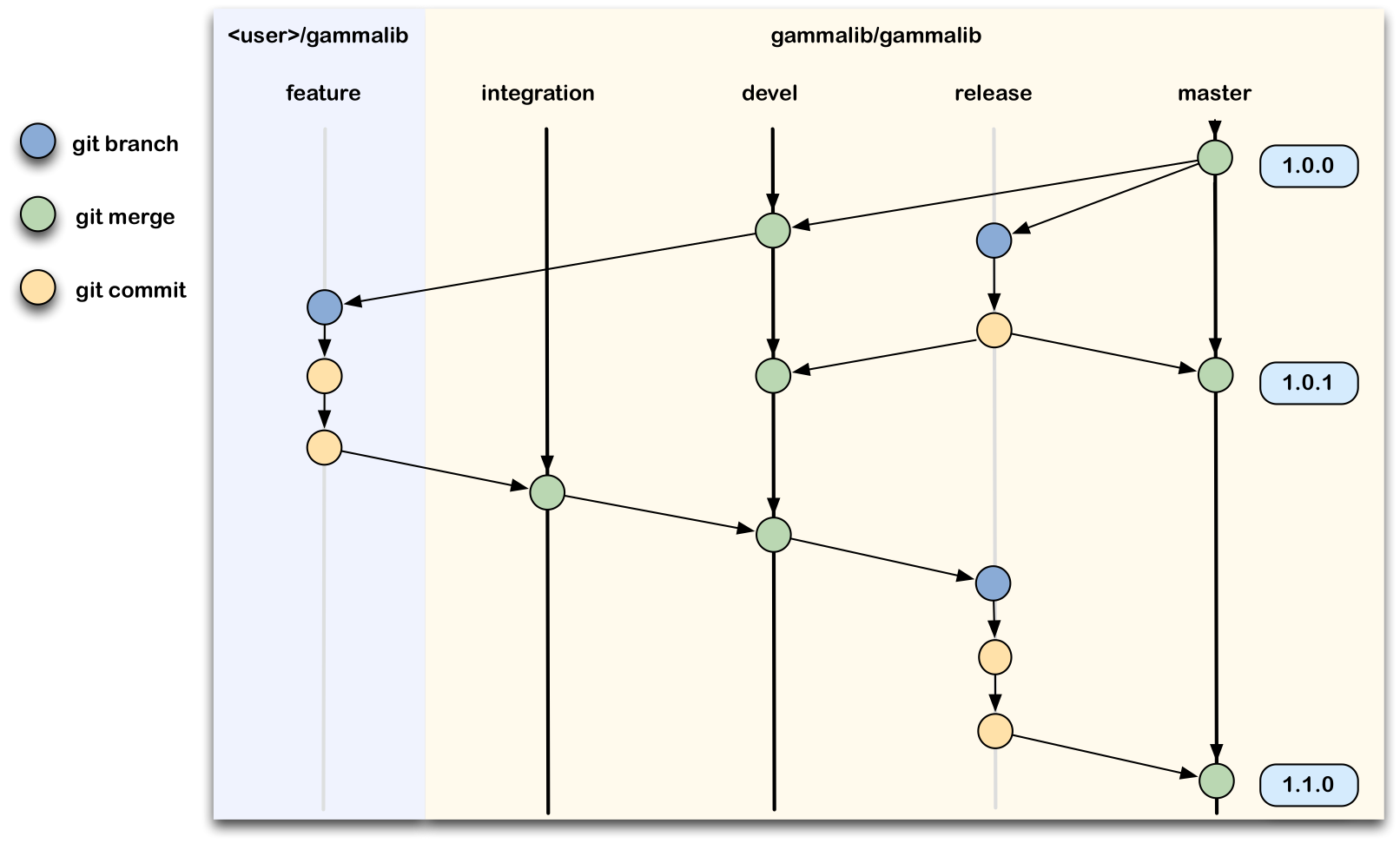 |
As the first step you need to create a fork of the project. Connect to GitLab with your Redmine user name and password (your user name on Redmine and GitLab is identical), select the GammaLib project and click on “Fork” (highlighted by the red box below):
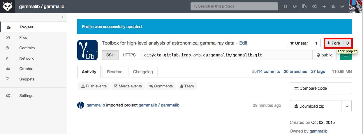 |
This brings you to a screen that invites you to fork (i.e. copy) the project to your user account. Click on your user (highlighted by the red box below):
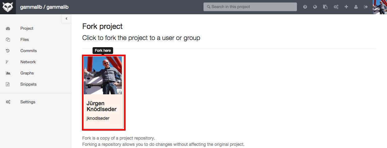 |
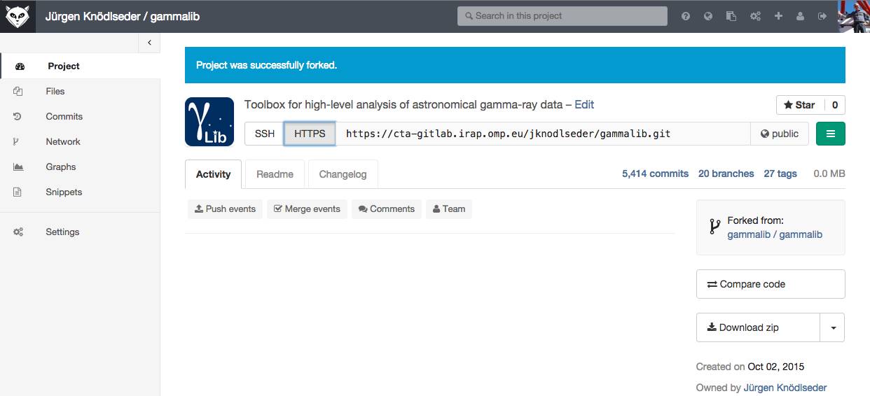 |
After a short while a fork will be created that now is under your ownership. You can access this fork through the HTTPS protocol at the address https://cta-gitlab.irap.omp.eu/<user>/gammalib.git where <user> needs to be replaced by your user name (your user name on Redmine and GitLab is identical). For the example below, you create a clone by typing in a shell:
$ git clone https://cta-gitlab.irap.omp.eu/jknodlseder/gammalib.git
$ git init
We recommend adding the main gammalib repository as a remote repository named upstream so that you can fetch the latest code version before you start a new feature:
$ git remote add upstream https://cta-gitlab.irap.omp.eu/gammalib/gammalib.git
To work on a feature or to correct a bug you step in the gammalib directory that was created after cloning and you create a new feature branch using
$ git pull upstream devel
$ git checkout -b 9101-correct-nasty-bug
The first command pulled in the latest changes from the main gammalib repository. Note that a branch name should always start with the number of the issue you work on and a short description what you actually are planning to do.
Suppose that there is a bug in the inst/cta/src/GCTAModelIrfBackground.cpp file. After correcting the bug you need to stage the change for commit using
$ git add inst/cta/src/GCTAModelIrfBackground.cppand then commit the change using
$ git commit -m "Fixed the nasty bug (#9101)"where the message in hyphens should be as detailed as possible (the example here is definitely not very good). Please also attach the issue number in the commit message. This allows tracking which issues were in fact fixed by a given commit.
Now you can push your change into the git repository using
$ git push origin 9101-correct-nasty-bugNote that the
origin argument specifies where to push the change (origin means to the same repository where you have cloned from), and the 9101-correct-nasty-bug argument gives the name of the branch you want to push.
You can now verify on GitLab that a new branch exists in your project:
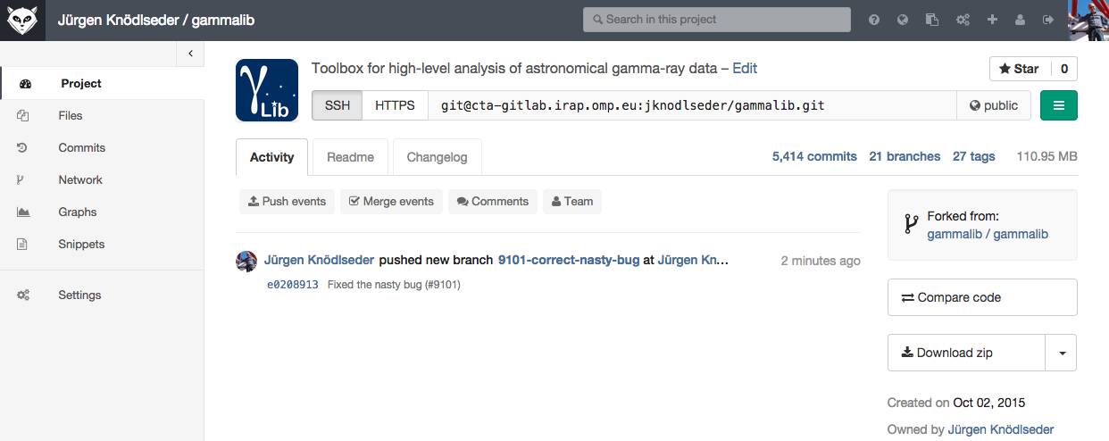 |
After having thoroughly checked your new code, and after having pushed the code into your git repository, you can now issue a pull request so that your change gets merged into the main code base (the so called “trunk”). For this you have to open the relevant issue in Redmine and put the status of the issue to “Pull request”:
 |
In the notes field please indicate where your change is. This means you should provide at least your user name on GitLab and the name of the feature branch. You could also copy/paste the HTTPS URL of your repository.
You should also describe in the notes field the changes or addition you made to the code. Explain what you have done. Say if there is anything you’d like particular attention for - like a complicated change or some code you are not happy with.
If you don’t think your request is ready to be merged, just say so in your pull request message. This is still a good way of getting some preliminary code review.
To delete a branch on GitLab, select the “Branches” tab and click on the wastebasket behind the branch you want to delete:
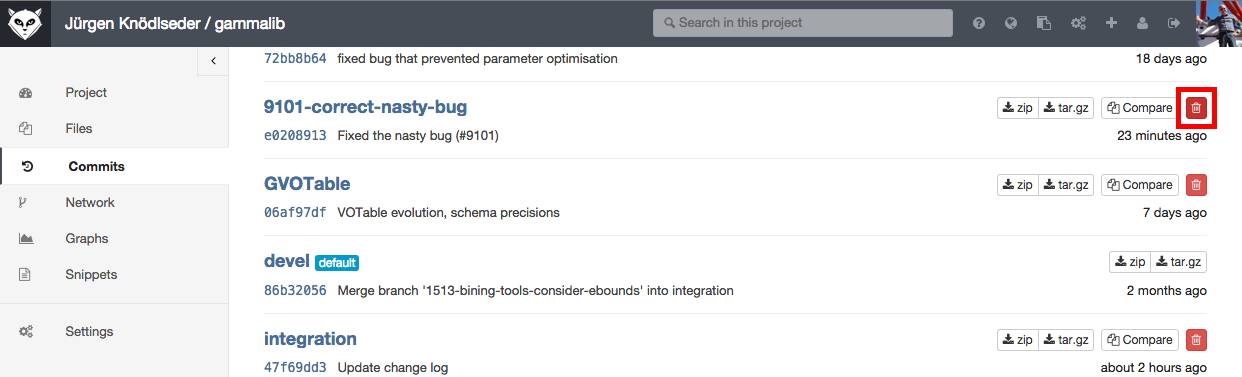 |
Updated over 8 years ago by
Any contributions to the GammaLib package, whether bug fixes, improvements to the documentation, or new functionality, can be done via pull requests. Pull requests are issued by changing the status of a GammaLib issue to Pull request.
As developer, you have two options for contribution code to the project:https://cta-git.irap.omp.eu/gammalibhttps://github.com/gammalib/gammalibWhich of the two to pick is a matter of taste. If you don’t know which to pick, use the irap one.
The only absolutely necessary configuration step is identifying yourself and your contact info:
$ git config --global user.name "Joe Public"
$ git config --global user.email "joe.public@gmail.com"
Please make sure that you specify your full name as user.name, do not use your abbreviated login name because this makes code modification tracking more cryptic.
In case that you get
error: SSL certificate problem, verify that the CA cert is OK.you may add
$ export GIT_SSL_NO_VERIFY=truebefore retrieving the code. Alternatively, you may type
$ git config --global http.sslverify "false"which disables certificate verification globally for your Git installation. The following sections cover the installation of the git software, the basic configuration, and links to resources to learn more about using git. If you use GitHub, you may also check the GitHub help pages which offer a great introduction to git and GitHub.
The following sections describe the configuration and the workflow for the central GammaLib repository.
The following sections describe the configuration and the workflow for the GitHub GammaLib repository.
Updated about 11 years ago by
Model functions will be called very often during a typical GammaLib analysis, hence evaluation of models need to be as efficient as possible. Here, pre computations are key. When possible, models should have a cache of precomputed values that will be used until parameters change. Note here that a check is much quicker than the evaluation of, for example, and exponential function. Thus we can afford some checks of this speeds up computations at the end.
Model locking is a possibility, that should be investigated. When a model is locked, it can be assumed that model parameters will not be modified. Having this capability will allow an efficient usage of pre computation. Model locking can for example be used in likelihood computations, and can help to speed up things considerably.
Two methods need to be implemented for each model (and probably model component): lock() and unlock(). When the lock() method has been called, and until a call of unlock(), the model can assume that parameters will not be changed. This allows to perform pre-computations on locking, and to use cached values until the model is unlocked. lock() can also call methods to perform pre computations.
Care has to be taken for numerical derivative computation, which will change parameters. Here we have to make sure that the model is unlocked before the derivative computation starts, and locked afterwards. If this is done too often, the gain of pre computation may be lost.le
It should be possible to link different parameters together. For this purpose, a link reference could be used, and by specifying this reference one could signal the GModels class that two or more parameters are in fact identical. The effective number of parameters will then be reduced.
Instead of specifying a parameter one may want to specify a function of parameters. The normal GModelPar would then be a simple case of the identity relation. Parameter functions could then allow to have one model scaling with s and another with 1-s. It also would allow to have for example an energy dependent parameter (not sure that this is really the same case). A parameter function may have other parameters or parameter functions as members. This will allow to implement functional relations of arbitrary complexity.
We may implement an abstract class GModelFunction that provides the interface for a parameter function. GModelPar would then be derived from this class as the implementation of the identiy function. A model may then have GModelPar members and GModelFunction members. Here an example:
GModelPar       m_ra;
GModelPar       m_dec;
GModelFunction* m_radius;
value method.GModelFunction should also have a gradient method that allows setting the gradient of the function parameters. The model class will set the gradient with respect to the function value, and the GModelFunction will compute the gradient of the function value with respect to the parameters. The GModelFunction::gradient method will multiply both for setting the parameter gradients.GModelFunction are either GModelPar parameters or GModelFunction classes. Functions can thus be nested, allowing the building of arbitrarily complex models.
<parameter name="RA" scale="1" ... />
<parameter name="DEC" scale="1" ... />
<function name="Radius" type="EnergyPowerLaw">
  <parameter name="Prefactor" scale="1" ... />
  <parameter name="Pivot" scale="1" ... />
  <function name="Index" type="sqrt">
    <parameter name="Index" scale="1" ... />
  </function>
</function>
Updated about 11 years ago by
The GModels container class holds a list of models. A model in the list is uniquely identified by its model name.
Updated about 11 years ago by
This class implements a sky model that is factorized into a spatial, a spectral and a temporal component. The factorization is given by
The spatial component describes the energy and time dependent morphology of the source. It satisfies
for all and
, hence the spatial component does not impact the spatially integrated spectral and temporal properties of the source.
The spectral component describes the spatially integrated time dependent spectral distribution of the source. It satisfies
for all , where
is the spatially and spectrally integrated total source flux. The spectral component does not impact the temporal properties of the integrated flux
.
The temporal component describes the temporal variation of the total integrated flux of the source.
Updated over 11 years ago by
The model has been validation by generating pull distributions using cspull. The validation has been done using ctools-00-06-00 and GammaLib-00-07-00.
An exponentially cut-off power law following the HESS Crab spectrum was used to generate mock data. Below the pull distributions for all fitted parameters (prefactor, spectral index, cut off energy and 2 background parameters) are shown for 10000 Monte Carlo samples for an exposure time of 18000 seconds. The deadtime correction factor was assumed to 0.95. The file kb_E_50h_v3 was used for the instrumental response function, data have been simulated for 0.1-100 TeV for an ROI of 5 deg.
 |
 |
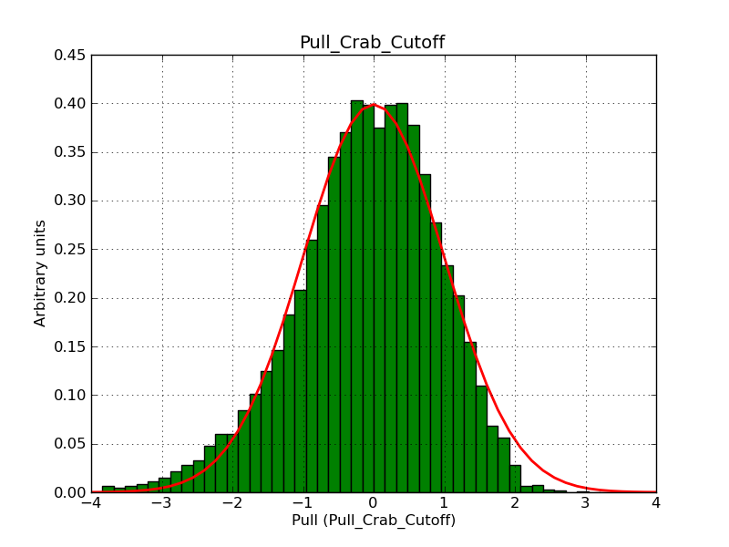 |
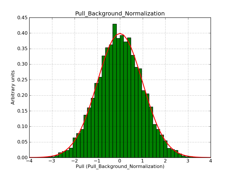 |
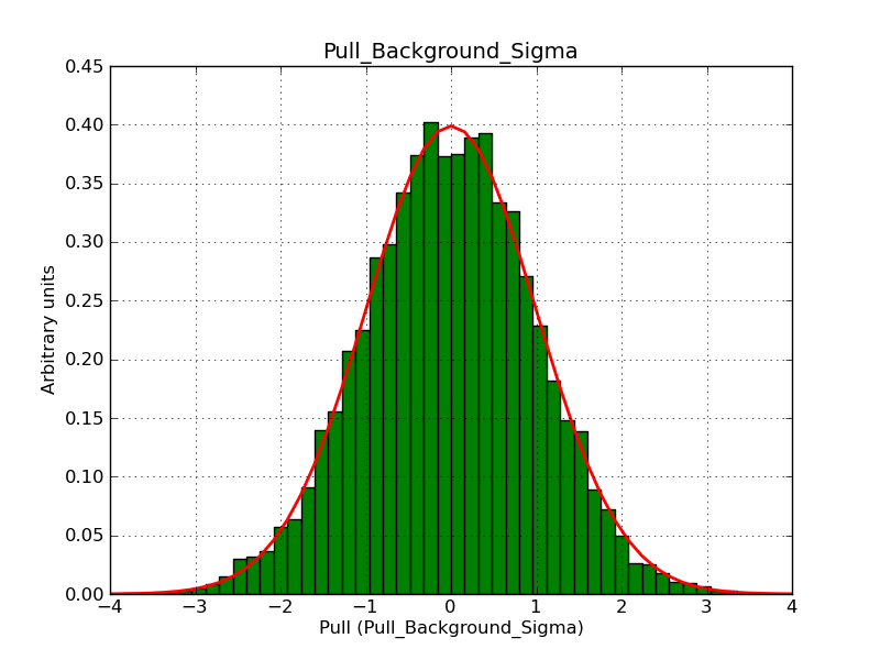 |
Apparently, there is some asymmetry in the uncertainty of the cut off energy. I guess that this comes from the fact that the cut off energy enters under the exponential in the spectral model, making the uncertainty inherently asymmetric.
Note: we may explore a model where instead of fitting the cut off energy, one fits the exponential of the cut off energy as parameter.
Updated over 10 years ago by
The model has been validation by generating pull distributions using cspull. The validation has been done using ctools-00-07-00 and GammaLib-00-08-00 pre-release versions.
The following model has been used:
<?xml version="1.0" standalone="no"?>
<source_library title="source library">
    <source name="Crab" type="PointSource">
        <spectrum type="Gaussian">
           <parameter name="Normalization" scale="1e-10" value="1.0"  min="1e-07" max="1000.0" free="1"/>
           <parameter name="Mean"          scale="1e6"   value="5.0"  min="0.01"  max="100.0"  free="1"/>
           <parameter name="Sigma"         scale="1e6"   value="1.0"  min="0.01"  max="100.0"  free="1"/>
        </spectrum>
        <spatialModel type="SkyDirFunction">
            <parameter free="0" max="360" min="-360" name="RA" scale="1" value="83.6331" />
            <parameter free="0" max="90" min="-90" name="DEC" scale="1" value="22.0145" />
        </spatialModel>
    </source>
</source_library>
Simulations has been done for 18000 seconds of CTA observation 0.1-10 TeV for an ROI of 5 deg. 10000 Monte Carlo samples have been drawn. Below the pull distributions, which look quite okay.
 |
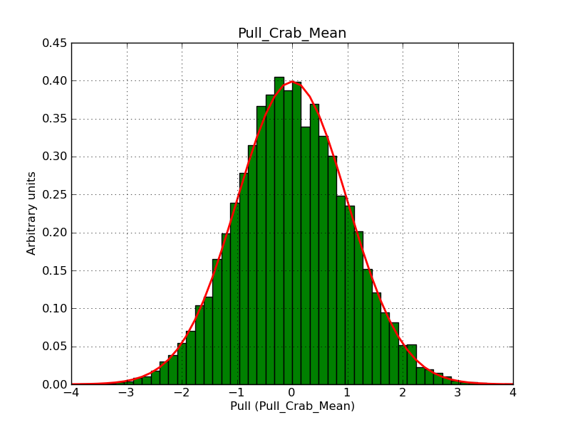 |
 |
Updated over 11 years ago by 
This class allows a spectrum definition with an energy-dependent index. It follows the formula:
: Normalisation at reference energy
: Index at reference energy
: Curvature
: Pivot energy (reference energy)
A first test of applying this model to real data from Fermi LAT and HESS is attached.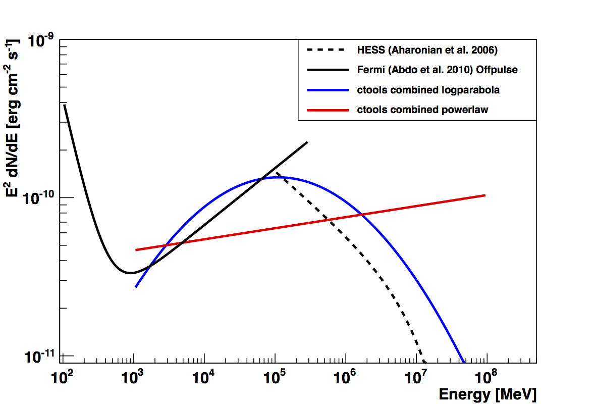
Below the code that is implemented in the Fermi-LAT ScienceTools. Note that the index and curvature are defined as positive values here, as the negative sign is explicitely implemented in the formula.
double LogParabola::value(optimizers::Arg & xarg) const {
   ::Pars pars(m_parameter);

   double energy = dynamic_cast<optimizers::dArg &>(xarg).getValue();
   double x = energy/pars[3];
   double my_value = pars[0]*std::pow(x, -(pars[1] + pars[2]*std::log(x)));
   return my_value;
}

double LogParabola::derivByParam(optimizers::Arg & xarg,
                                 const std::string & paramName) const {
   ::Pars pars(m_parameter);

   double energy = dynamic_cast<optimizers::dArg &>(xarg).getValue();
   double x = energy/pars[3];
   double logx = std::log(x);
   double dfdnorm = std::pow(x, -(pars[1] + pars[2]*logx));

   int iparam = -1;
   for (unsigned int i = 0; i < pars.size(); i++) {
      if (paramName == pars(i).getName()) {
         iparam = i;
      }
   }

   if (iparam == -1) {
      throw optimizers::ParameterNotFound(paramName, getName(),
                                          "LogParabola::derivByParam");
   }

   enum ParamTypes {norm, alpha, beta, Eb};
   switch (iparam) {
   case norm:
      return dfdnorm*m_parameter[norm].getScale();
   case alpha:
      return -pars[0]*logx*dfdnorm*m_parameter[alpha].getScale();
   case beta:
      return -pars[0]*logx*logx*dfdnorm*m_parameter[beta].getScale();
   case Eb:
      return value(xarg)/pars[3]*(pars[1] + 2.*pars[2]*logx)
         *m_parameter[Eb].getScale();
   default:
      break;
   }
   return 0;
}
the method GModelSpectralLogParabola::mc(GEnergy emin, GEnergy emax, GRan ran) returns a random energy following the LogParabola distribution. The following plots have been produced using normalised LogParabola with the Parameters index=-2, curvature=+-0.2 and E0=100MeV. 100000 Events have been simulated. Red lines show the underlying LogParabola model while green lines correspond to the respective powerlaws which are used as function for the "rejection sampling method". 

Updated over 11 years ago by
The model has been validation by generating pull distributions using cspull. The validation has been done using ctools-00-06-00 and GammaLib-00-07-00.
A power law following the HESS Crab spectrum was used to generate a 10 node spectral node model. The energy values of the 10 nodes are:
0.5, 0.834, 1.391, 2.321, 3.871, 6.458, 10.772, 17.969, 29.974, and 50 TeV.
Below the pull distributions for all fitted parameters (10 spectral nodes and 2 background parameters) for 10000 Monte Carlo samples for an exposure time of 1800 seconds. The deadtime correction factor was assumed to 0.95. The file kb_E_50h_v3 was used for the instrumental response function, data have been simulated for 0.1-100 TeV for an ROI of 5 deg. The script crab_05_50_10_deadc095_t1800_n10000.sh and the model crab_05_50_10.xml was used to produce the results.
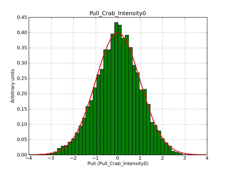 |
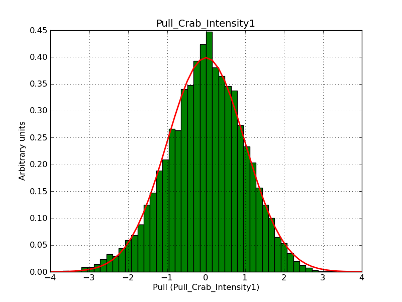 |
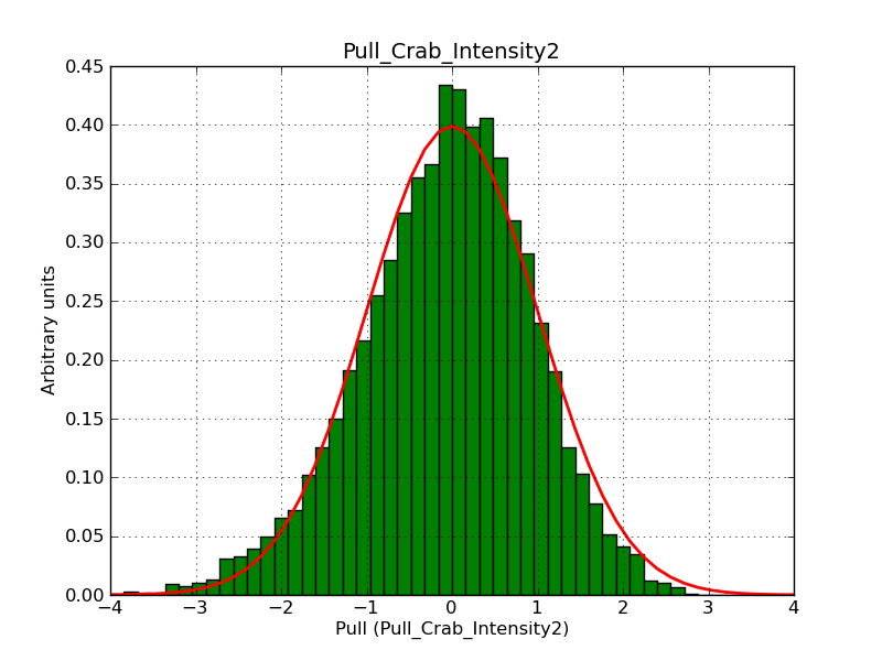 |
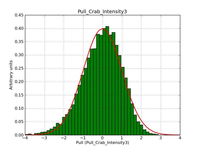 |
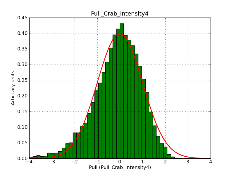 |
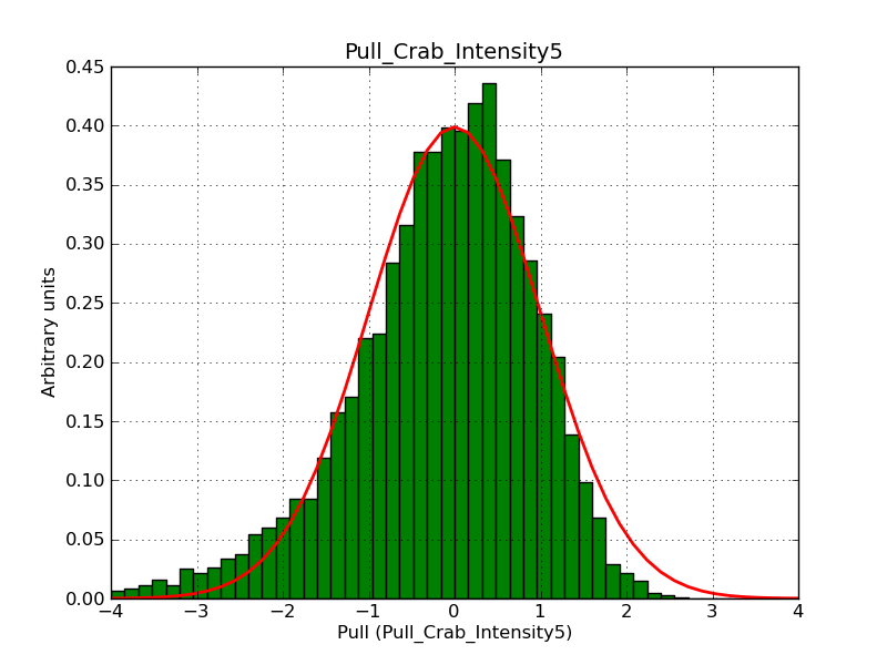 |
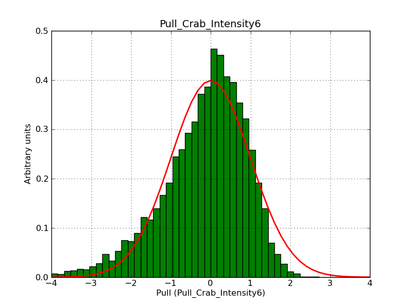 |
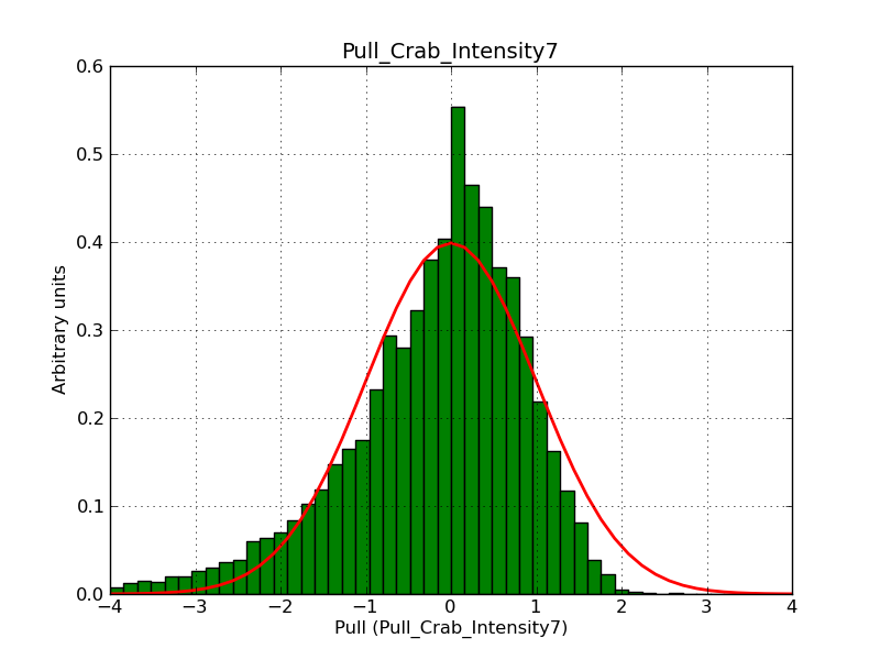 |
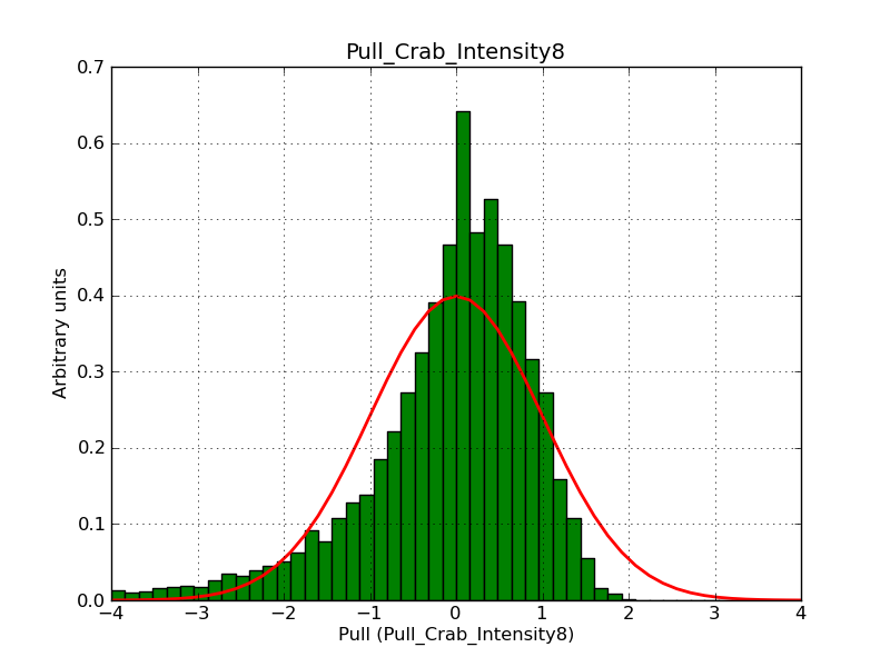 |
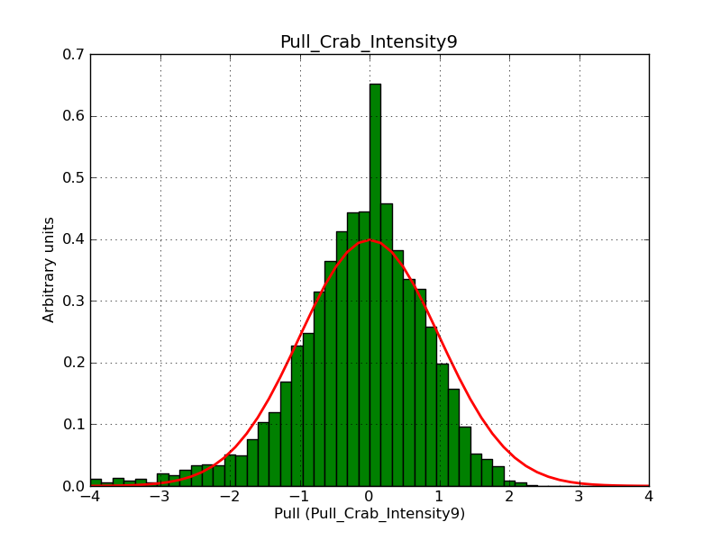 |
 |
 |
Obviously, with increasing energies the distribution becomes asymmetric. This is due to the small number of counts simulation for large energies, leading to a deviation from Gaussian statistics at high energies. Increasing the exposure time to 18000 seconds reduces the effect. The results for simulation for an exposure time of 18000 seconds are shown below.
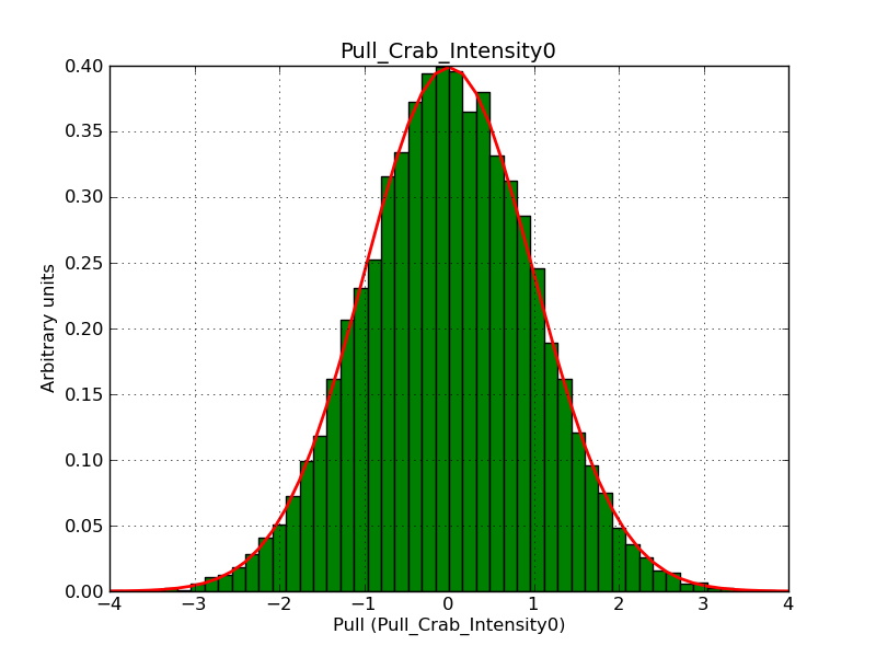 |
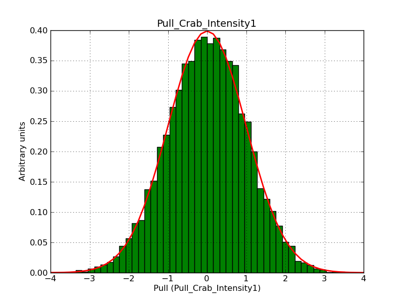 |
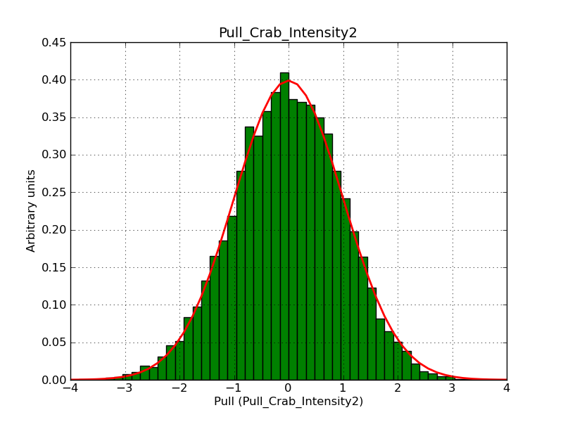 |
 |
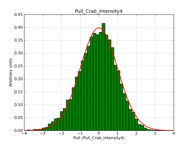 |
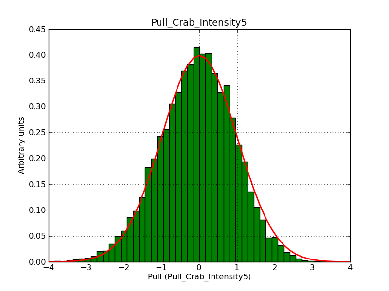 |
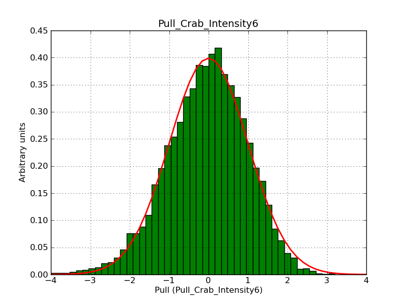 |
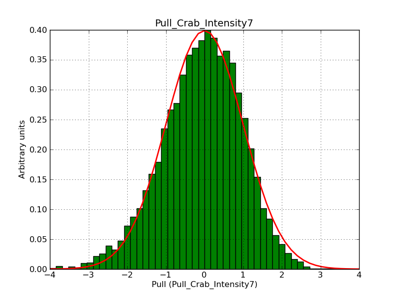 |
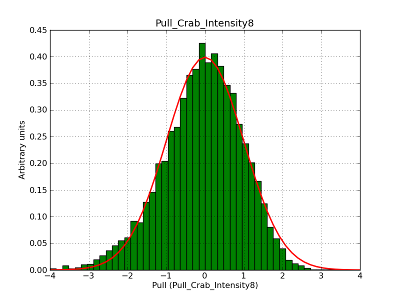 |
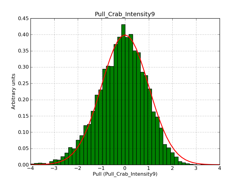 |
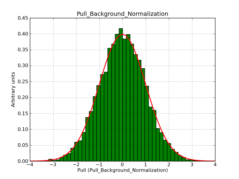 |
 |
Updated over 11 years ago by
The model has been validation by generating pull distributions using cspull. The validation has been done using ctools-00-06-00 and GammaLib-00-07-00.
A power law following the HESS Crab spectrum was used to generate mock data. Below the pull distributions for all fitted parameters (integral flux, spectral index, source position and 2 background parameters) are shown for 10000 Monte Carlo samples for an exposure time of 18000 seconds. The deadtime correction factor was assumed to 0.95. The file kb_E_50h_v3 was used for the instrumental response function, data have been simulated for 0.1-100 TeV for an ROI of 5 deg.
 |
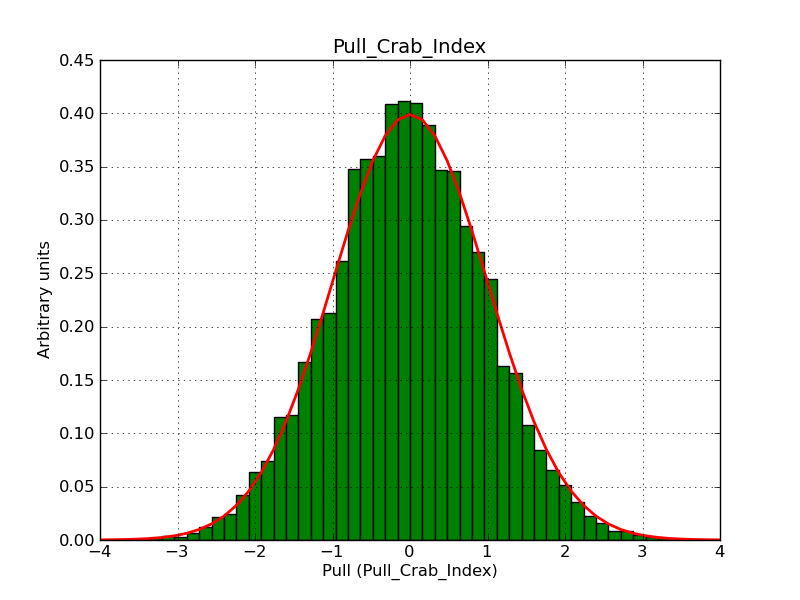 |
 |
 |
 |
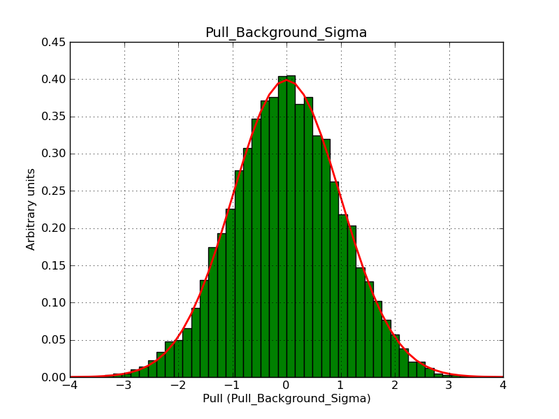 |
Updated over 11 years ago by
The model has been validation by generating pull distributions using cspull. The validation has been done using ctools-00-06-00 and GammaLib-00-07-00.
A power law following the HESS Crab spectrum was used to generate mock data. Below the pull distributions for all fitted parameters (integral flux, spectral index, source position and 2 background parameters) are shown for 10000 Monte Carlo samples for an exposure time of 18000 seconds. The deadtime correction factor was assumed to 0.95. The file kb_E_50h_v3 was used for the instrumental response function, data have been simulated for 0.1-100 TeV for an ROI of 5 deg.
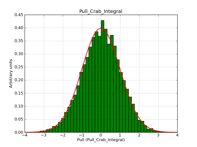 |
 |
 |
 |
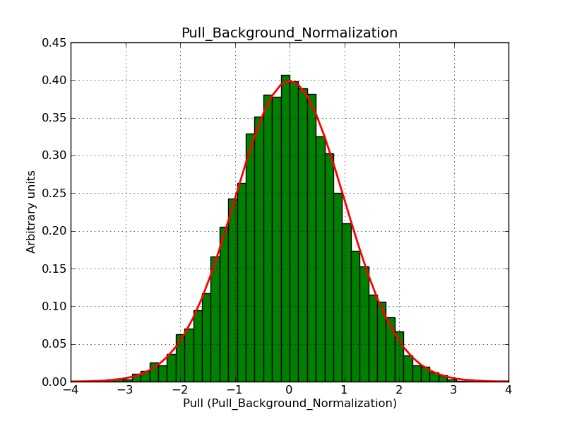 |
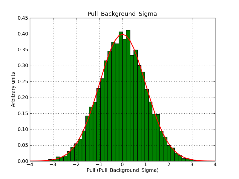 |
Updated over 11 years ago by Anonymous
See OpenMP page for configuration of parallelization options.
In the GObersation class, OpenMP is used to parallelize the eval method in the optimizer part (GObersation::optimizer::eval). Loop iterations are split and dealt to the differents threads. Each thread has their own variable to avoid conflict with shared variable ( as m_value, m_npred or m_gradient ), this working variables are store temporarily in vectors which are loop over at the end of iterations to update shared variables.
In this first test, fitting was executed on real data with 50 observations.
The computer used for this test is Kepler, a server with 48 cores.
")
We can notice in this chart some irregularities with computation time caused by the number of iterations which is not constant ( between 23 and 34).
The algorithm is not very stable and stop condition of fitting is very precise ( 1e-6). With round-off error, number of iterations can change with number of thread and depend of the execution order.
To delete dependence on number of iterations, the next chart divide the time by it.

Here the line is smoothest but after 10 threads performance does not evolute a lot.
An other test with 20 observations.
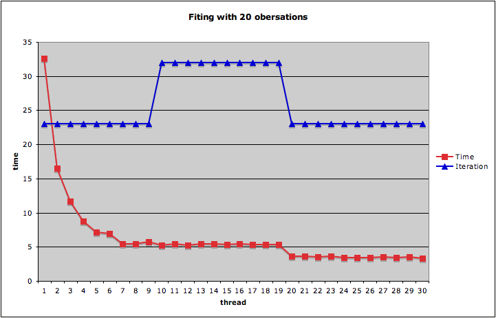
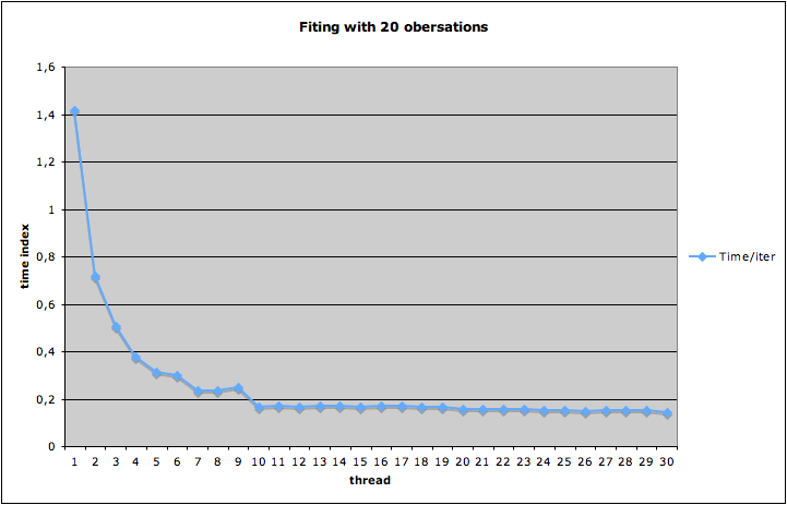
Updated about 11 years ago by
The GObservations container class holds a list of observations. For a given instrument, an observation in the list is uniquely identified by its observation identifier.
Updated almost 12 years ago by
This class implements the Levenberg Marquard function optimizer.
Here a list of useful links concerning the Levenberg Marquard optimizer:
GOptimizerLM comes from)Updated over 11 years ago by
The GRegion class is an abstract virtual base class that describes a region on the sky in arbitrary coordinates. Here a draft of the class definition:
class GRegion {
    virtual void        clear(void) = 0;
    virtual GRegion*    clone(void) const = 0;
    virtual bool        isin(const GSkyDir& dir) const = 0;
    virtual void        read(const GXmlElement& xml) = 0;
    virtual void        write(GXmlElement& xml) const = 0;
    virtual std::string print(void) const = 0;
}
The GRegions class is a container to hold derived classes of type GRegion. Here a draft of the class definition:
class GRegions {
    GRegion&       operator[](const int& index);
    const GRegion& operator[](const int& index) const;
    void           clear(void);
    int            size(void) const;
    void           append(const GRegion& region, const bool& include = true);
    void           insert(const int& index, const GRegion& region, const bool& include = true);
    void           extend(const GRegions& regions);
    void           pop(const int& index = -1);
    void           load(const std::string& filename);
    void           save(const std::string& filename) const;
    void           read(const GXml& xml);
    void           write(GXml& xml) const;
    bool           isin(const GSkyDir& dir) const = 0;
    std::string    print(void) const;
}
Note that the append, insert, extend and pop methods are standard methods for container classes (although insert, extend and pop is so far rarly implemented in GammaLib). The load and save methods should act on XML files, the read and write methods on GXml objects (which are basically opened XML files). We may also implement methods for loading and saving ds9 region files (e.g. load_ds9 and save_ds9).
The GRegions container could then be used as follows to select pixels from a sky map:
GRegions regions("my_preferred_regions.xml");
GSkymap  map("my_nice_sky_map.fits");
GSkymap  selected = map.select(regions);
selected.save("my_selected_pixels.fits");
In the same way it can be used internally by the CTA event cube class, as the event cube data are stored in a GSkymap object.
We can of course invent whatever format we like, but it would be worth checking if some XML format exists already for regions, e.g. in the virtual observatory.
Updated over 11 years ago by
GRegistry is the interface class for all registry classes in GammaLib. The class in an abstract base class which defines the methods that all registry classes are required to implement. Below the interface definition
class GRegistry {
public:
    virtual ~GRegistry(void) {}
    virtual int         size(void) const = 0;
    virtual std::string name(const int& index) const = 0;
    virtual std::string print(void) const = 0;
};
Updated over 11 years ago by
The GSkyDir class implements a direction on the sky, given either in equatorial (FK5 J2000) or Galactic coordinates.
The coordination transformation (a simple rotation) is checked in test_GSky.py in Test.test_fk5_to_galactic().
The gammalib results agree with PyAST within 10 milli-arcseconds for the whole sky.
Once we consider adding astronomical time and coordinate functionality to gammalib, this might be a useful reference:
https://github.com/astropy/coordinates-benchmark
Updated over 11 years ago by
The GTime class is intended to handle times in an abstract way.
The existing implementation tries to incorporate different time systems in a single class. The implementation is definitely not satisfactory, but it satisfies the current needs (which are not high as no time conversion is in fact used). In the long run, the class should be redefined to handle various time systems efficiently (see Feature #284).
Here some thoughts about a possible new implementation.
The GTime class can be the base class for instrument specific time classes. One option is that GTime is not abstract, i.e. it can be used without any instrument information. The class has just a single member, which is the time in seconds in UTC with a well defined zero point (for example January 1st, 2000, this is to be defined). The class has then basic access methods that allow setting and returning of the time in seconds, days, MJD and JD. Maybe also some string formating should be supported.
Instrument specific time classes are then derived from the GTime class and implement conversion classes from the instrument specific time to UTC. The conversion can be done via constructors or specific conversion methods. It remains to be seen whether these conversion constructors and methods exist only for the derived classes, or whether they overload base class methods.
Alternatively, the instrument specific classes could store the time in the instrument time reference, and then implement the proper conversion methods to go to UTC. This avoids time conversion when they are not necessary (in most cases). Time conversion would thus only exist on an instrument specific level. The GTime could then even be abstract, and a GUTCTime class could be added to handle general times in the UTC time reference.
GGti. GGti is a general class, but it should also handle instrument specific times. There a several solutions to this:
GTime for storing times in instrument specific reference. This is more a kluge that works if the GGti is only used within the instrument specific frame, which we can never be sure, however. The advantage is that there is little overhead, the disadvantage is that we never can be sure what time reference is in the GTime. This is prone to errors.GGti. This looks complicated and implies a bunch of time conversions.At the end it seems that the abstract solution with an instrument specific registry seems to be the best. Each time can then say in which reference it is, and we can fall back to GUTCTime if we need an instrument independent time.
The abstract GTime class would then have the pure virtual methods:
virtual double jd(void) const = 0;
virtual double mjd(void) const = 0;
virtual double secs(void) const = 0;
virtual double days(void) const = 0;
virtual void   jd(const double& time) = 0;
virtual void   mjd(const double& time) = 0;
virtual void   secs(const double& time) = 0;
virtual void   days(const double& time) = 0;
jd and mjd methods perform time conversion, the secs and days return the time in native format.
But what is the real advantage of having instrument specific times? Can’t we just convert always to the same time reference, and then just go with this?
I’m no longer convinced that the abstract base class scheme is really what we want. One reason is that time manipulation becomes more complicated. For example, we can’t simply write
GTime tstart;
GTime tstop;
...
GTime time = tstop - tstart;
GCTATime tstart;
GCTATime tstop;
...
GUTCTime time = tstop - tstart;
In fact, the only advantage of having derived classes is that the reference time can be stored statically, and also complicated time transformations can be coded. This would allow handling for example the specific onboard time formats for some satellites. But do we really need this for high-level analysis?
It seems better to keep the actual structure and to store the time reference information in the GGti class. We may even add a GTimeReference class for this, so that time references can be delt with in any context.
The GTime holds the time in a GammaLib specific time reference. The time is stored in a double precision value in seconds.
The following methods are implemented to access or modify the time value:
double      jd(void) const;               //!< Return time in Julian Days
double      mjd(void) const;              //!< Return time in Modified Julian Days
double      secs(void) const;             //!< Return time in seconds (GammaLib specific reference time)
double      days(void) const;             //!< Return time in days (GammaLib specific reference time)
std::string utc(void) const;              //!< Return time as UTC string
void        jd(const double& time);       //!< Set time in Julian Days
void        mjd(const double& time);      //!< Set time in Modified Julian Days
void        secs(const double& time);     //!< Set time in seconds (GammaLib specific reference time)
void        days(const double& time);     //!< Set time in days (GammaLib specific reference time)
void        utc(const std::string& time); //!< Set time from UTC string
The time reference is implemented by a GTimeReference class. This class should provide methods to transform the time in a given reference to the GammaLib specific reference time. The class should be able to read (write) the time reference information from (to) an OGIP FITS HDU.
The time reference can be stored in the GGti class, allowing the automatic conversion of the time values into the GammaLib specific time reference. Keeping this information in the GGti class allows then writing back the time in the specified time reference.
The Systeme International (SI) second is defined as the duration of 9,192,631,770 cycles of radiation corresponding to the transition between two hyperfine levels of the ground state of cesium 133.
Universal Time 1 (UT1) is the time system based on the rotation of the earth. Because of changes in the earth’s rotation rate, in UT1 a day is not exactly 86400 s.
Coordinated Universal Time (UTC) provides a uniform-rate time system referenced to atomic clocks where a day is 86400 s. To keep UT1 and UTC within 0.9 s, a leap second is added to UTC as needed, typically every few years (see the USNO leap second history). UTC is the same as Greenwich Mean Time (GMT) or Zulu time (for the military).
Leap seconds can cause errors in measurements that straddle the addition of a leap second. The Terrestrial Time (TT) is a uniform rate time system referenced to the geoid without leap seconds. Effectively, TT time is greater than UTC time by a number that increases by 1 second every time a leap second is added to UTC. Below a table of leap seconds for different periods in time:| Period | Leap seconds |
| 1990 Jan. 1 - 1991 Jan. 1 | 25s |
| 1991 Jan. 1 - 1992 Jul. 1 | 26s |
| 1992 Jul. 1 - 1993 Jul 1 | 27s |
| 1993 Jul. 1 - 1994 Jul. 1 | 28s |
| 1994 Jul. 1 - 1996 Jan. 1 | 29s |
| 1996 Jan. 1 - 1997 Jul. 1 | 30s |
| 1997 Jul. 1 - 1999 Jan 1 | 31s |
| 1999 Jan. 1 - 2006 Jan 1 | 32s |
| 2006 Jan. 1 - 2009 Jan 1 | 33s |
| 2009 Jan. 1 - 2012 Jul 1 | 34s |
| 2012 Jul. 1 - | 35s |
Another method of avoiding leap seconds over a time span of a number of years is to use the number of seconds relative to a reference time. This is the method that astrophysical missions often use, where the number of seconds is called 'Mission Elapsed Time’ (MET). Because MET and TT are both continuous uniform-rate time systems, MET and TT will always be offset from each other by a constant. Note that the time system should be included in specifying a reference time (e.g., whether the reference time is midnight on a particular date in the TT or UTC system).
The Global Positioning System (GPS) uses its own continuous uniform-rate time system that is related by a constant offset (13.184 s) to TT.
The Julian Date (JD) is the number of days since Greenwich mean noon on January 1, 4713 B.C.E. Since JD is a large number—midnight at the beginning of January 1, 2008, corresponds to JD=2454466.5—and our calendar uses midnight as the beginning and end of a calendar day, the Modified Julian Date (MJD) has been defined as MJD=JD-2400000.5. Midnight (i.e., 0h:0m:0s) differs between the UTC and TT systems, and therefore one should specify whether a JD or MJD date is in the UTC or TT system.
Below
| Date (UTC) | MJD (UTC) | MJD (TT) | TT-UTC | Notes |
| January 1, 1998 | 63.184 sec | XMM-Newton reference | ||
| January 1, 2001 (UTC) | 51910.0 | 51910.0007428703703703703 | 64.184 sec | Fermi-LAT reference |
| January 1, 2010 (UTC) | 55197.0 | 55197.000766018518519 | 66.184 sec | GammaLib reference |
This Wiki page summarizes the organization and development efforts planned for the HESS sprint #1 that will take place at IRAP (Toulouse, France) from Monday June 24 (noon) to Friday June 28 (noon).
See the https://cta-redmine.irap.omp.eu/projects/ctools/wiki/Coding_sprints page for information on later coding sprints.
The purpose of the sprint is to extend the GammaLib and ctools to allow the analysis of data from Cherenkov telescopes in a way currently adopted by the HESS/VERITAS/MAGIC collaborations: the ON and OFF technique, which can be used in different ways. The objectives are concept validation and cross-checking with the existing analysis pipelines. Our initial goal is to provide support for a point source spectral analysis for data taken in wobble mode using background estimates from reflected regions.
The meeting will start with some introduction to GammaLib and ctools development, followed by a common software coding session (for the spirit of the meeting see https://en.wikipedia.org/wiki/Sprint_(software_development)).
An initial discussion about the project can be found in GammaLib-ctools_AddTradAnaMethods.pdf. This was followed by a code structure proposal presented in GammaLib-ctools_AddTradAnaMethods_2.pdf. The first objective of the meeting is to fix the code structure and interfaces, before filling in the required functionalities.
The following people have attended the code sprint:
An informal program for the coding sprint is:
The list of features and tasks dealt with during the HESS sprint #1 is:
The latter action about XSPEC actually shares many tasks with what is needed for classical analysis (in the form of PHA and ARF data notably), so it was decided to consider both developments at the same time.
An outline of the things we’d like to implement can be obtained from the virtual scripts posted in #570.
The philosophy eventually adopted is to have Gammalib providing mostly the necessary objects (such as sky regions or ON-OFF data container), while the action is done by specific ctools. This allows for modularity. On use and extension to other classical analysis methods, it may appear that some functionalities may need to be shifted from ctools to gammalib.
Taken from Christoph...
The fit statistic function should live on GObservation (may be extended to whole gammalib).
GObservations.optimizer(LevMarOpt) is a method on the GObservations container that calls an external minimizer.
In the container there could be one Fermi GObservation, one HESS spectral observation, … any kind of data set.
Create per-run IRFs that contain the full information for the whole field of view:
1. full-enclosure effective area as a function of X, Y, logE
2. PSF as a function of X, Y, logE, theta2
integrate to 1 along theta2 axis
3. Energy resolution as a function of X, Y, logEtrue, logEreco
integrate to 1 along logEreco axis
Notes:
1. The IRFs are stored as 3D and 4D FITS arrays.
2. There is no reason to pre-define the ranges / binning of the axes.
The IRFs are used as lookups, they do not define the analysis data space.
Linear interpolation in the range and linear or constant extrapolation outside should be OK.
3. X and Y has WCS info attached (i.e. pixel ↔ world transformation is easily possible)
4. logE and theta2 binning is defined in FITS table extensions (example: Fermi diffuse model file)
Check that the FITS effective area, PSF and energy resolution matches HAP / ParisAnalysis values.
Open questions:
- Store IRFs as ND array or as a FITS table with one row (X and Y pixel coordinates, WCS info stored separately)
- Should IRFs be attached to the event list as extra HDUs or in separate FITS files?
- alternative for PSF: use triple-Gauss instead of theta2 histogram?
- support analysis without energy resolution (i.e. effective area as a function of reco energy)?
- safe energy cut?
- background?
The meeting will take place in room 225-226 (in the basement of IRAP-Roche building). Coffee breaks at 11:00 and 16:30.
How to come to IRAP:
From the airport:
- Take the shuttle bus. You can find it at 50m from one of the exit gate (depending on where you exit, you may have to follow the road and pass the taxi line)
- Tickets probably cannot be purchased on the bus but at an office that is located next to the exit gate (only at night can they be purchased on the bus)
- The fare is 5€ and cover the shuttle bus and the public transportation downtown for a 1h duration.
- If you need/want to go to your hotel first, you’ll have to alight at “Jean Jaurès” which is the most central stop (up to you to check where your hotel is)
- Otherwise, you can alight at the first stop of the shuttle bus which is “Compans Caffarelli”
- From “Jean Jaurès” or “Compans Caffarelli”, take the subway line B (there are only two lines: A/red and B/yellow, and they cross only at Jean Jaurès).
- Take the subway direction “Ramonville”
- Alight at “Faculté de pharmacie”
- From here you can either walk (10-15min) or take the bus.
- The bus stop is on your right when you exit the subway station. Take bus line 78 and alight at “LAAS”.
- Then you are a few 100m away from IRAP, use the attached map.
The map shows you the way from subway station to IRAP if you walk. The bus takes the same way except at the beginning, and will drop you slightly before the roundabout.
Updated over 11 years ago by
Checkout the branch into which you want to copy the file
$ git checkout destination
$ git checkout other_branch file_to_copy.txt
Updated over 11 years ago by
Ideally, one would like to avoid casts, as they indicate a poorly defined interface. However, sometimes one still would like to have a cast. An example is the GInstDir class, which defines an abstract direction in the instrument system. Sometimes, the direction has nothing to do with a position on the sky (for example for the SPI telescope on INTEGRAL which is a non-imaging telescope), sometimes the instrument direction is identical to a sky position (for all imaging telescopes). So how can we get out of GInstDir object the sky direction? We need a cast.
A cast can be implement as a class extension in the SWIG interface. Here a cast for the GCTAInstDir class:
%extend GCTAInstDir {
    GCTAInstDir(GInstDir* dir) {
        GCTAInstDir* ptr = dynamic_cast<GCTAInstDir*>(dir);
        if (ptr != NULL) {
            return (ptr->clone());
        }
        else {
            throw GException::bad_type("GCTAInstDir(GInstDir*)", "GInstDir not of type GCTAInstDir");
        }
    }
};
It is used for example as in
instdir = GCTAInstDir(dir)
Note that the extension does in fact not really implement a cast, but it provides a deep copy of the instrument direction. The method also verifies that the cast is valid.
Updated over 11 years ago by
A one-dimensional function can be integrated using the
GIntegral class. To compute proceed as follows:
You need first to define the kernel function by deriving a class from the base class
GFunction. In the following example, we define the function , where
is a parameter of the function:
class function : public GFunction {
public:
    function(double a) : m_a(a) {}
    double eval(double x) { return m_a*x; }
protected:
    double m_a;  //!< A parameter needed by the function
};
eval(x) method that will be used to evaluate The numerical integral is then computed using the Romberg integration method provided by the GIntegral class. The following example illustrates how to proceed:
function f(47.0);
GIntegral integral(&f);
integral.eps(1.0e-8);
double xmin = 1.0;
double xmax = 2.0;
result = integral.romb(xmin, xmax);
Updated over 3 years ago by
gdb --args ctlike inobs=file.fits ...
(gdb) where
(gdb) bt
(gdb) bt full
(gdb) break ctobservation.cpp:129
(gdb) s (or step)      # Step to next source line
(gdb) n (or next)      # Step to next source line in the current file
(gdb) p obs
(gdb) p obs.m_models
(gdb) p obs.m_models.m_models
(gdb) p **(obs.m_models.m_models._M_impl._M_start)@1    # Print one element of vector
(gdb) p **(obs.m_models.m_models._M_impl._M_start+1)    # Print 2nd element of vector
$ ulimit -c unlimited
$ ssh root@dirac (or whatever machine)
# sysctl -w kernel.core_pattern=/tmp/core-%e.%p.%h.%t
kernel.core_pattern = /tmp/core-%e.%p.%h.%t
# exit
$ gdb -c /tmp/core-gsrvy.8920.dirac.1596483045 (or whatever the filename of the core dump)
(gdb) symbol-file /home/knodlseder/install/bin/gsrvy (or whatever path to the binary)
(gdb) sharedlibrary
(gdb) where
Updated over 3 years ago by
Valgrid is a very useful tool for finding bottle necks in the execution of code and to identify where actually the type is spent.
valgrind --tool=callgrind --dump-instr=yes --collect-jumps=yes gsrvy (args)
Mark the code zone using some macros
#include <valgrind/callgrind.h>

int main()
{
  foo1();
  CALLGRIND_START_INSTRUMENTATION;
  CALLGRIND_TOGGLE_COLLECT;
  bar1();
  CALLGRIND_TOGGLE_COLLECT;
  CALLGRIND_STOP_INSTRUMENTATION;
  foo2();
  foo3();
}
valgrind --tool=callgrind --dump-instr=yes --collect-jumps=yes --collect-atstart=no --instr-atstart=no gsrvy (args)
If the callgrind.out.* file is empty call
callgrind_control -d [hint [PID/Name]]where hint is an arbitrary string you can optionally specify to later be able to distinguish profile dumps.
Check whether instrumentation is turned on using
callgrind_control -b
You can also decide to switch instrumentation on using
callgrind_control -i on(and switching off again by specifying “off” instead of “on”).
Use the kcachegrind GUI to visualise the results.
Updated over 3 years ago by
free
watch -n 5 free -m
vmstat
Either of
valgrind --tool=massif gsrvy
valgrind --tool=massif --massif-out-file=massif.out.%p gsrvy
valgrind --tool=massif --pages-as-heap=yes gsrvy
This produces an output file, for example
massif.out.51550 (the second variant is useful for forked processes, the third variant assures that all memory allocated is traced). To visualise the output, typems_print massif.out.51550In the graphs produced,
ki is “kilo instructions executed” as a measure of time.Note that the gsrvy execution does not need to finish, ctrl-C stops execution and produces the relevant output files.
Using valgrind a call tree can be generated using
valgrind --tool=massif --xtree-memory=full gsrvywhich can then be inspected using
kcachegrind. The call tree filename is xtmemory.kcg.[pid] which can be opened with kcachegrind.
To investigate the memory usage or call tree while an executable is running, valgrind needs to be used through a gdb server. In one console, start gsrvy using
valgrind --tool=massif --xtree-memory=full --vgdb=yes --vgdb-error=0 gsrvyThis will inform about the command sequence to be used in
gdb in a second terminal. Start now gdb in a second terminal:gdb gsrvy (gdb) target remote | /usr/libexec/valgrind/../../bin/vgdb --pid=59212Now the valgrind job can be controlled from gdb.
Starting the job:
(gdb) continue
Creating an intermediate memory call tree:
(gdb) ctrl-C
(gdb) monitor xtmemory
(gdb) continue
See https://www.valgrind.org/docs/manual/ms-manual.html#ms-manual.monitor-commands for all
monitor commands.
Note: Instead of starting gdb one can also send commands to valgrind using the vgdb program:
vgdb --pid=59212 xtmemory [<filename> default xtmemory.kcg.%p.%n] requests Massif tool to produce an xtree heap memory report.
vgdb --pid=59212 snapshot [<filename>] requests to take a snapshot and save it in the given <filename> (default massif.vgdb.out).
vgdb --pid=59212 detailed_snapshot [<filename>] requests to take a detailed snapshot and save it in the given <filename> (default massif.vgdb.out).
vgdb --pid=59212 all_snapshots [<filename>] requests to take all captured snapshots so far and save them in the given <filename> (default massif.vgdb.out).
vgdb --pid=59212 v.info memory
Updated over 11 years ago by
The instructions here are adapted from http://book.git-scm.com/2_installing_git.html
$ sudo apt-get install git-core
$ sudo yum install git-core
There are several ways to install git on Mac. The easiest is to simply download the OS X installer (git-osx-installer). If you have MacPorts installed, you can also do:
$ sudo port install git-core
$ sudo apt-get install git
Updated about 4 years ago by
Updated over 11 years ago by Anonymous
Here Jenkins specification for JUnit XML files.
Found here: https://svn.jenkins-ci.org/trunk/hudson/dtkit/dtkit-format/dtkit-junit-model/src/main/resources/com/thalesgroup/dtkit/junit/model/xsd/junit-4.xsd
<?xml version="1.0" encoding="UTF-8" ?>
<xs:schema xmlns:xs="http://www.w3.org/2001/XMLSchema">

    <xs:element name="failure">
        <xs:complexType mixed="true">
            <xs:attribute name="type" type="xs:string" use="optional"/>
            <xs:attribute name="message" type="xs:string" use="optional"/>
        </xs:complexType>
    </xs:element>

    <xs:element name="error">
        <xs:complexType mixed="true">
            <xs:attribute name="type" type="xs:string" use="optional"/>
            <xs:attribute name="message" type="xs:string" use="optional"/>
        </xs:complexType>
    </xs:element>

    <xs:element name="properties">
        <xs:complexType>
            <xs:sequence>
                <xs:element ref="property" maxOccurs="unbounded"/>
            </xs:sequence>
        </xs:complexType>
    </xs:element>

    <xs:element name="property">
        <xs:complexType>
            <xs:attribute name="name" type="xs:string" use="required"/>
            <xs:attribute name="value" type="xs:string" use="required"/>
        </xs:complexType>
    </xs:element>

    <xs:element name="skipped" type="xs:string"/>
    <xs:element name="system-err" type="xs:string"/>
    <xs:element name="system-out" type="xs:string"/>

    <xs:element name="testcase">
        <xs:complexType>
            <xs:sequence>
                <xs:element ref="skipped" minOccurs="0" maxOccurs="1"/>
                <xs:element ref="error" minOccurs="0" maxOccurs="unbounded"/>
                <xs:element ref="failure" minOccurs="0" maxOccurs="unbounded"/>
                <xs:element ref="system-out" minOccurs="0" maxOccurs="unbounded"/>
                <xs:element ref="system-err" minOccurs="0" maxOccurs="unbounded"/>
            </xs:sequence>
            <xs:attribute name="name" type="xs:string" use="required"/>
            <xs:attribute name="assertions" type="xs:string" use="optional"/>
            <xs:attribute name="time" type="xs:string" use="optional"/>
            <xs:attribute name="classname" type="xs:string" use="optional"/>
            <xs:attribute name="status" type="xs:string" use="optional"/>
        </xs:complexType>
    </xs:element>

    <xs:element name="testsuite">
        <xs:complexType>
            <xs:sequence>
                <xs:element ref="properties" minOccurs="0" maxOccurs="1"/>
                <xs:element ref="testcase" minOccurs="0" maxOccurs="unbounded"/>
                <xs:element ref="system-out" minOccurs="0" maxOccurs="1"/>
                <xs:element ref="system-err" minOccurs="0" maxOccurs="1"/>
            </xs:sequence>
            <xs:attribute name="name" type="xs:string" use="required"/>
            <xs:attribute name="tests" type="xs:string" use="required"/>
            <xs:attribute name="failures" type="xs:string" use="optional"/>
            <xs:attribute name="errors" type="xs:string" use="optional"/>
            <xs:attribute name="time" type="xs:string" use="optional"/>
            <xs:attribute name="disabled" type="xs:string" use="optional"/>
            <xs:attribute name="skipped" type="xs:string" use="optional"/>
            <xs:attribute name="timestamp" type="xs:string" use="optional"/>
            <xs:attribute name="hostname" type="xs:string" use="optional"/>
            <xs:attribute name="id" type="xs:string" use="optional"/>
            <xs:attribute name="package" type="xs:string" use="optional"/>
        </xs:complexType>
    </xs:element>

    <xs:element name="testsuites">
        <xs:complexType>
            <xs:sequence>
                <xs:element ref="testsuite" minOccurs="0" maxOccurs="unbounded"/>
            </xs:sequence>
            <xs:attribute name="name" type="xs:string" use="optional"/>
            <xs:attribute name="time" type="xs:string" use="optional"/>
            <xs:attribute name="tests" type="xs:string" use="optional"/>
            <xs:attribute name="failures" type="xs:string" use="optional"/>
            <xs:attribute name="disabled" type="xs:string" use="optional"/>
            <xs:attribute name="errors" type="xs:string" use="optional"/>
        </xs:complexType>
    </xs:element>

</xs:schema>
Updated almost 12 years ago by
Below the XML format that is output by JUnit:
<?xml version="1.0" encoding="UTF-8"?>
<testsuites disabled="" errors="" failures="" name="" tests="" time="">
    <testsuite disabled="" errors="" failures="" hostname="" id=""
        name="" package="" skipped="" tests="" time="" timestamp="">
        <properties>
            <property name="" value=""/>
            <property name="" value=""/>
        </properties>
        <testcase assertions="" classname="" name="" status="" time="">
            <skipped/>
            <error message="" type=""/>
            <error message="" type=""/>
            <failure message="" type=""/>
            <failure message="" type=""/>
            <system-out/>
            <system-out/>
            <system-err/>
            <system-err/>
        </testcase>
        <system-out/>
        <system-err/>
    </testsuite>
</testsuites>
Releases
GitLab
GitHub
SourceForge
GammaLib - A new framework for the analysis of Astronomical Gamma-Ray Data
Updated about 11 years ago by
The method-call overhead is the time spent in passing arguments to a method and retrieving the return value. Normally, the method-call overhead is only relevant for methods that perform very little computations, so that a substantial fraction of the time is spent by setting up the method call.
To illustrate the method-call overhead, check the small attached program arguments.cpp / arguments.hpp. The program can be compiled using for example
$ g++ -o arguments arguments.cppThe program tests passing 5 or 15 arguments in 3 different ways:
| 5 | 15 | |
| By value | 0.86 | 1.73 |
| By reference | 0.70 | 1.64 |
| Using a structure | 0.30 | 0.34 |
Obviously, passing a single structure as argument produces the smallest method-call overhead. Passing by reference is a little faster than passing by value, even for int values.
The general rules derived from this experiment are:| 5 | 15 | |
| By value | 1.02 | 2.15 |
| By reference | 0.83 | 2.19 |
| Using a structure | 0.46 | 0.98 |
Updated almost 10 years ago by 
This pages summarizes the most frequently encountered problems of GammaLib developers. If you encountered a problem and think it’s worth reporting it, including the solution, don’t hesitate to add it to this page.
On Mac OS X, using macports you might encounter a problem related to swig:
gammalib/app_wrap.cpp:2034:11: warning: explicitly assigning a variable of type 'int’ to itself [-Wself-assign]
res = SWIG_AddCast(res);
~~ ^ ~~
gammalib/app_wrap.cpp:11549:55: error: use of undeclared identifier 'SWIG_PyInstanceMethod_New’
{ (char *)"SWIG_PyInstanceMethod_New", (PyCFunction)SWIG_PyInstanceMethod_New, METH_O, NULL}
It is not clear to me where this problem is coming from, but might be related to file permission. If you run a “sudo make” instead of a “make”, the compilation proceeds without any problems. I’ve traced the problem as far as to the files, where SWIG_AddCast() is declared. The files are called pycomplex.py, pyprimtypes.py and pyrun.swg and are located in the /opt/local/share/swig/3.0.2/python folder of macports.
Updated almost 12 years ago by
Updated about 11 years ago by
Strict naming conventions should be followed throughout GammaLib to make the library coherent, easy to use, and non-conflicting with other packages.
GammaLib classes shall start with an upper case G, followed by a human understandable name of which the first letter is in upper case. Examples are
GEnergy
GModels
GEventBin
GEvent => GEventBin
GFitsImage => GFitsImageDouble
GammaLib functions names should be as close as possible to functions names used commonly in C++. For example, to take the sine of every element of a GammaLib vector, the sin name is used:
GVector elements;
...
GVector sin_of_elements = gammalib::sin(elements);
gammalib.
Global variables in GammaLib should start with g_. The rest of the name should be as descriptive and specific as possible.
Constants used throughout GammaLib shall also be placed in the gammalib namespace.
To avoid naming conflicts, GammaLib shall never use internally any using directive, but shall always put the namespace in front of the function or constant.
Updated over 8 years ago by
Updated over 11 years ago by Anonymous
OpenMp is the API used by GammaLib to paralellize some parts of the code.
IMPORTANT: if GammaLib is compiled with parallelization, openmp flag is required ( -fopenmp with GCC) for C++ code using it.
Else errors like this will appear:
/libgamma.so: undefined reference to `GOMP_critical_end'
/libgamma.so: undefined reference to `omp_get_thread_num'
/libgamma.so: undefined reference to `omp_get_num_threads'
/libgamma.so: undefined reference to `GOMP_sections_start'
/libgamma.so: undefined reference to `GOMP_parallel_start'
/libgamma.so: undefined reference to `GOMP_sections_end'
/libgamma.so: undefined reference to `GOMP_critical_start'
/libgamma.so: undefined reference to `GOMP_parallel_end'
/libgamma.so: undefined reference to `GOMP_sections_next'
/libgamma.so: undefined reference to `GOMP_barrier'
documentation :
http://www.openmp.org/mp-documents/spec25.pdf
http://en.wikipedia.org/wiki/OpenMP
http://software.intel.com/en-us/articles/getting-started-with-openmp/
It is possible to configure paralellization with environment variable.
The usefull is OMP_NUM_THREADS which sets the maximum number of threads to use during execution. For example:export OMP_NUM_THREADS=8
To see all environment variables : https://computing.llnl.gov/tutorials/openMP/#EnvironmentVariables
Updated over 8 years ago by
This page provides performance verification information for the various GammaLib release versions. Performance verification information is collected per date. The applicable GammaLib version is quoted in the first column of the table.
| GammaLib version | ||||
| 0.10.0 | Spectral unbinned (2015-06) | Spectral stacked (2015-07) | Spatial unbinned (2015-08) | Spatial stacked (2015-08) |
Updated about 11 years ago by
print() method so that information about the object can be obtained by the user. The print() method will return a string that can be dumped on a terminal or into a log file. The print() method will taken an integer argument that specified the chattiness of information that should be put into the string. The following chatter level are defined:
GChatter type, which is an enumeration that can take the following values:
SILENTTERSENORMALEXPLICITVERBOSEHere some guidelines for the implementation of each chatter level.
At this level the print() method should in general return an empty string, unless that some error information is to be printed.
At this level, the print() method should only provide a couple of lines. In particular, the content of a class (i.e. observations, events, photons, ...) should not be displayed.
This is the normal information level. The print() method should provide all information relevant that is relevant for a gamma-ray analysis. For example, the observation container will display summary information for each observation.
At this level, the print() method should provide also information about the detailed content of an object. For example, the GPhotons class will print all photons it contains.
At this level, the print() method should also display information that is useful for debugging, such as internal cache states, etc.
Updated over 11 years ago by
As developer, you have two options for sharing your code with the project: either you use the central GammaLib repository https://cta-git.irap.omp.eu/gammalib or you use a fork on Github (https://github.com/gammalib/gammalib). In the following, the workflow for both options is explained.
A first step you need to create a fork of gammalib on GitHub. You need to do this only once. The instructions here are very similar to the instructions at http://help.github.com/fork-a-repo/ - please see that page for more details. We’re repeating some of it here just to give the specifics for the GammaLib project, and to suggest some default names.
If you don’t have a GitHub account, go to the GitHub page, and make one.
You then need to configure your account to allow write access - see the Generating SSH keys help on GitHub Help.
jknodlseder)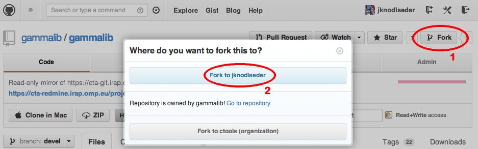
After a short pause, you should find yourself at the home page for your own forked copy of GammaLib (in this example https://github.com/jknodlseder/gammalib).
As next step, you have to setup the fork on your local computer. You also need to do this only once.
Use the command
$ git clone git@github.com:<user>/gammalib.git
remote: Counting objects: 22147, done.
remote: Compressing objects: 100% (4911/4911), done.
remote: Total 22147 (delta 17346), reused 21980 (delta 17179)
Receiving objects: 100% (22147/22147), 80.25 MiB | 42 KiB/s, done.
Resolving deltas: 100% (17346/17346), done.
to clone the GammaLib repository from GitHub. Here,
<user> is your GitHub user name (jknodlseder in the example above).
Now connect to the GitHub GammaLib repository using
$ cd gammalib
$ git remote add upstream git://github.com/gammalib/gammalib.git
upstream here is just the arbitrary name we’re using to refer to the main GammaLib repository.
Note that we’ve used git:// for the URL rather than git@. The git:// URL is read only. This means we that we can’t accidentally (or deliberately) write to the upstream repo, and we are only going to use it to merge into our own code.
You may verify that the connection has been established with
$ git remote -v
origin    git@github.com:jknodlseder/gammalib.git (fetch)
origin    git@github.com:jknodlseder/gammalib.git (push)
upstream    git://github.com/gammalib/gammalib.git (fetch)
upstream    git://github.com/gammalib/gammalib.git (push)
Your fork is now set up correctly, and you are ready to hack away.
It may sound strange, but deleting your own master branch can help reduce confusion about which branch you are on. See deleting master on github for details.
To delete the master branch, type
$ git checkout devel
Already on 'devel'

$ git branch -D master
error: branch 'master' not found.

$ git push origin :master
To git@github.com:jknodlseder/gammalib.git
 - [deleted]         master
Don’t worry if you get the message
error: branch 'master' not found., this just signals that you never checked out the master branch.
This section gives a summary of the workflow once you have successfully forked the repository, and details are given for each of these steps in the following sections.
devel branch, and start a new feature branch from that.536-refactor-database-code.devel or any other branches into your feature branch while you are working.devel, consider Rebasing on devel.This way of working helps to keep work well organized, with readable history.
devel¶From time to time you should fetch the latest changes from the devel branch from GitHub.
$ git fetch upstream
From git://github.com/gammalib/gammalib
 * [new branch]      devel      -> upstream/devel
 * [new branch]      master     -> upstream/master
 * [new branch]      release    -> upstream/release
This will pull down any commits you don’t have, and set the remote branches to point to the right commit.
When you are ready to make some changes to the code, you should start a new branch. We call this new branch a feature branch.
The name of a feature branch should always start with the Redmine issue number, followed by a short informative name that reminds yourself and the rest of us what the changes in the branch are for. For example 735-add-ability-to-fly, or 123-bugfix. If you don’t find a Redmine issue for your feature, create one.
Create the feature branch using
$ git fetch upstream
From git://github.com/gammalib/gammalib
 * [new branch]      devel      -> upstream/devel
 * [new branch]      master     -> upstream/master
 * [new branch]      release    -> upstream/release

$ git branch 007-my-new-feature upstream/devel
Branch 007-my-new-feature set up to track remote branch devel from upstream.

$ git checkout 007-my-new-feature
Switched to branch '007-my-new-feature'
The first command makes sure that the latests commits are fetched from the GitHub repository, the second command creates the feature branch, and the last command switches to the feature branch.
Generally, you will want to keep your feature branches on your public GitHub fork. To do this, you git push this new branch up to your GitHub repo:
$ git push origin 007-my-new-feature
Total 0 (delta 0), reused 0 (delta 0)
To git@github.com:jknodlseder/gammalib.git
 * [new branch]      007-my-new-feature -> 007-my-new-feature
007-my-new-feature is related to the 007-my-new-feature branch in the GitHub repo.
Here a typical command sequence, where a file is added, the change is committed, and the commit is pushed to the repository.
$ git add my_new_file

$ git commit -am 'NF - some message'
[007-my-new-feature 403d7d2] NF - some message
 1 files changed, 1 insertions(+), 0 deletions(-)
 create mode 100644 my_new_file

$ git push origin
Counting objects: 4, done.
Delta compression using up to 4 threads.
Compressing objects: 100% (2/2), done.
Writing objects: 100% (3/3), 303 bytes, done.
Total 3 (delta 1), reused 0 (delta 0)
To git@github.com:jknodlseder/gammalib.git
   04bab2c..403d7d2  007-my-new-feature -> 007-my-new-feature
devel¶Eventually, the devel branch has advanced while you developed the new feature. In this case, you should rebase your code before asking for merging. Rebasing is done using:
$ git fetch upstream
remote: Counting objects: 5, done.
remote: Compressing objects: 100% (1/1), done.
remote: Total 3 (delta 2), reused 3 (delta 2)
Unpacking objects: 100% (3/3), done.
From git://github.com/gammalib/gammalib
   04bab2c..ccba491  devel      -> upstream/devel

$ git checkout 007-my-new-feature
Already on '007-my-new-feature'
Your branch and 'upstream/devel' have diverged,
and have 1 and 1 different commit(s) each, respectively.

$ git branch tmp 007-my-new-feature

$ git rebase upstream/devel
First, rewinding head to replay your work on top of it...
Applying: NF - some message
Here we created a backup of
007-my-new-feature into tmp for safety.
When all looks good you can delete your backup branch using
$ git branch -D tmp
Deleted branch tmp (was 403d7d2).
If your feature branch is already on GitHub and you rebase, you will have to force push the branch; a normal push would give an error. Use this command to force-push:
$ git push -f origin 007-my-new-feature
Counting objects: 8, done.
Delta compression using up to 4 threads.
Compressing objects: 100% (5/5), done.
Writing objects: 100% (6/6), 611 bytes, done.
Total 6 (delta 3), reused 0 (delta 0)
To git@github.com:jknodlseder/gammalib.git
 + 403d7d2...816ac2c 007-my-new-feature -> 007-my-new-feature (forced update)
When you are ready to ask for someone to review your code and consider a merge, change the status of the issue you’re working on to Pull Request:
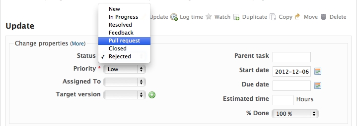
In the notes field, describe the set of changes, and put some explanation of what you’ve done. Say if there is anything you’d like particular attention for - like a complicated change or some code you are not happy with.
If you don’t think your request is ready to be merged, just say so in your pull request message. This is still a good way of getting some preliminary code review.
$ git checkout devel
Switched to branch 'devel'

$ git branch -D 007-my-new-feature
Deleted branch 007-my-new-feature (was 816ac2c).

$ git push origin :007-my-new-feature
To git@github.com:jknodlseder/gammalib.git
 - [deleted]         007-my-new-feature
Note the colon : before
007-my-new-feature. See also: http://github.com/guides/remove-a-remote-branch
$ git clone https://<manager>@cta-git.irap.omp.eu/gammalib
Cloning into 'gammalib'...
Password:
remote: Counting objects: 22150, done.
remote: Compressing objects: 100% (7596/7596), done.
remote: Total 22150 (delta 17330), reused 18491 (delta 14497)
Receiving objects: 100% (22150/22150), 80.12 MiB | 192 KiB/s, done.
Resolving deltas: 100% (17330/17330), done.
where
<manager> is the user name of the integration manager (e.g. jknodlseder).
Now connect to the GitHub repository of the developer using
$ cd gammalib

$ git remote add developer git://github.com/developer/gammalib.git

$ git remote -v
developer    git://github.com/developer/gammalib.git (fetch)
developer    git://github.com/developer/gammalib.git (push)
origin    https://jknodlseder@cta-git.irap.omp.eu/gammalib (fetch)
origin    https://jknodlseder@cta-git.irap.omp.eu/gammalib (push)
developer here is the GitHub user name of the developer from which we want to integrate changes.
$ git fetch developer
remote: Counting objects: 4, done.
remote: Compressing objects: 100% (1/1), done.
remote: Total 3 (delta 1), reused 3 (delta 1)
Unpacking objects: 100% (3/3), done.
From git://github.com/developer/gammalib
 * [new branch]      007-my-new-feature -> developer/007-my-new-feature
 * [new branch]      INCLUDES_to_AM_CPPFLAGS -> developer/INCLUDES_to_AM_CPPFLAGS
 * [new branch]      devel      -> developer/devel
 * [new branch]      pep8       -> developer/pep8
 * [new branch]      release    -> developer/release
 * [new branch]      integration -> developer/integration

$ git branch 007-my-new-feature --track developer/007-my-new-feature
Branch 007-my-new-feature set up to track remote branch 007-my-new-feature from developer.

$ git checkout 007-my-new-feature
Switched to branch '007-my-new-feature'
If there are only a few commits, consider rebasing to upstream:
$ git fetch origin
$ git rebase origin/devel
If there are a longer series of related commits, consider a merge instead:
$ git merge --no-ff origin/develNote the
--no-ff above. This forces git to make a merge commit, rather than doing a fast-forward, so that these set of commits branch off devel then rejoin the main history with a merge, rather than appearing to have been made directly on top of devel.
Now, in either case, you should check that the history is sensible and you have the right commits:
$ git log --oneline --graph
$ git log -p origin/devel..
The first line above just shows the history in a compact way, with a text representation of the history graph. The second line shows the log of commits excluding those that can be reached from
devel (origin/devel), and including those that can be reached from current HEAD (implied with the .. at the end). So, it shows the commits unique to this branch compared to devel. The -p option shows the diff for these commits in patch form.
$ git checkout integration

$ git merge 007-my-new-feature
Updating ccba491..562f236
Fast-forward
 my_new_file |    1 +
 1 files changed, 1 insertions(+), 0 deletions(-)
 create mode 100644 my_new_file

$ git commit -am 'Merged 007-my-new-feature.'

$ git push origin
Password:
Counting objects: 4, done.
Delta compression using up to 4 threads.
Compressing objects: 100% (2/2), done.
Writing objects: 100% (3/3), 306 bytes, done.
Total 3 (delta 1), reused 0 (delta 0)
remote: To https://github.com/gammalib/gammalib.git
remote:    ccba491..562f236  integration -> integration
remote:  * [new branch]      github/integration -> github/integration
To https://jknodlseder@cta-git.irap.omp.eu/gammalib
   ccba491..562f236  integration -> integration
The push will automatically launch the integration pipeline on Jenkins.
You should verify the all checks are passed with success.
$ git checkout devel
Switched to branch 'devel'

$ git merge integration
Updating ccba491..562f236
Fast-forward
 my_new_file |    1 +
 1 files changed, 1 insertions(+), 0 deletions(-)
 create mode 100644 my_new_file

$ git push origin
Updated over 9 years ago by
Citing https://wiki.python.org/moin/Python2orPython3, Python 2.x is legacy, Python 3.x is the present and future of the language. Having said this, most distribution still come today with Python 2.x, while some new distributions now feature Python 3.x. Obviously, GammaLib needs to support both. Most of the compatibility work will be done by SWIG, but there are a number of special features the developer has to be aware of.
Here a couple of rules to follow:print "My text" in a Python script, use print("My text"). print() is a function in Python.Python 3.x introduces two different division types: true division and floor division. In Python 2.x, division of two integers gave an integer, in Python 3.x it gives a floating point value. To get the old behavior back, floor division indicated by the floor division operator // should be used, i.e.
a = 1
b = 2
int_div = a // b
__idiv__ or __div__ methods implemented. In Python 3.x, __idiv__ or __div__ do not exist anymore but are now replaced by __itruediv__ or __truediv__ for true division and __ifloordiv__ or __floordiv__ for floor division.
Unfortunately, up to now SWIG (version 3.0.2) does not seem to support the two Python 3.x division types, and the operator/= results in the Python 2.x __idiv__ method that is not recognized by Python 3.x. To make the Python interface both compatible to Python 2.x and Python 3.x, both the __idiv__ and __itruediv__ methods should be implemented for unary division, and both the __div__ and __truediv__ methods should be implemented for binary division. As example, the following extension exists for GSkymap:
// Python 2.x operator/=
GSkymap __idiv__(const GSkymap& map) {
    self->operator /=(map);
    return (*self);
}
// Python 3.x operator/=
GSkymap __itruediv__(const GSkymap& map) {
    self->operator /=(map);
    return (*self);
}
For more reading on this topic, see http://legacy.python.org/dev/peps/pep-0238/. For a discussion about the SWIG fix, see https://github.com/swig/swig/pull/136.
Updated about 8 years ago by
Release notes
Download
Documentation
Performance
Submission guidelines
Contributing to GammaLib
Git workflow
Coding Conventions
Development Guidelines
Development Notes
Development HowTo
Deployment
Continuous Integration
Code release
Sidebar
Updated over 8 years ago by
The following plots summarize the pull distributions for the spatial models obtained using an unbinned analysis.
| Point source |  |
 |
|||
| Disk |  |
 |
 |
||
| Gaussian | 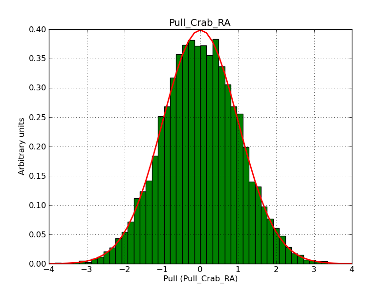 |
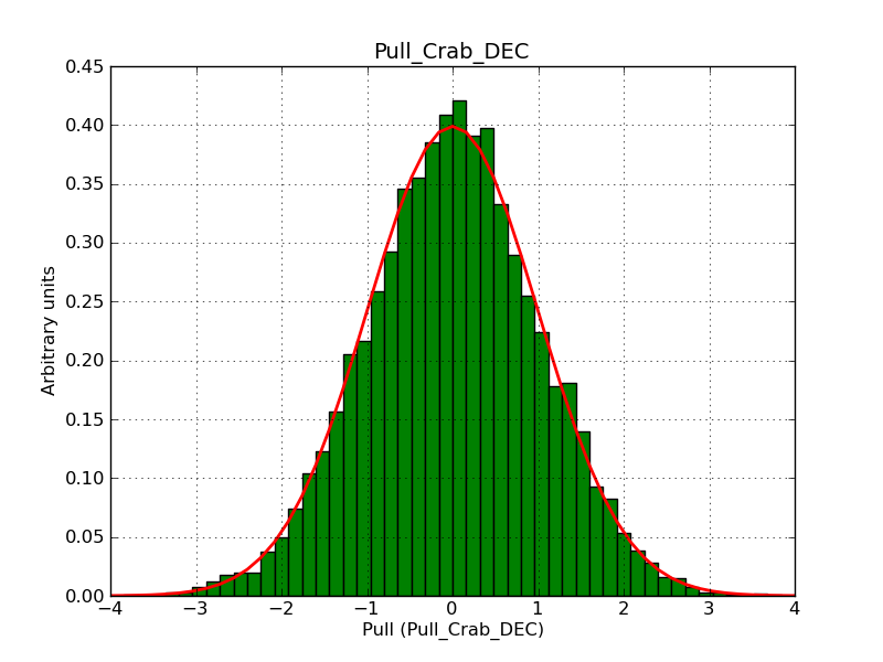 |
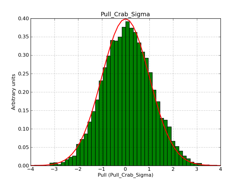 |
||
| Shell | |||||
| Elliptical Disk |  |
 |
 |
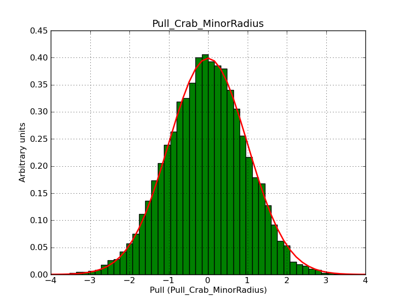 |
 |
| Elliptical Gaussian |
The following plot summarize the corresponding spectral components:
| Point source |  |
 |
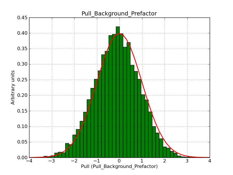 |
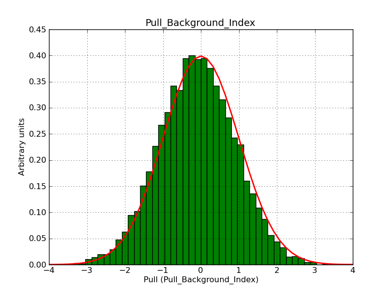 |
| Disk |  |
 |
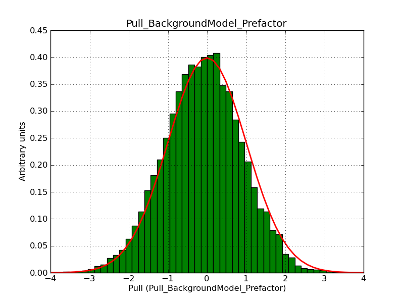 |
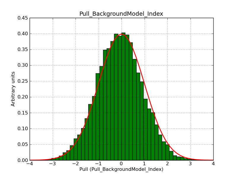 |
| Gaussian |  |
 |
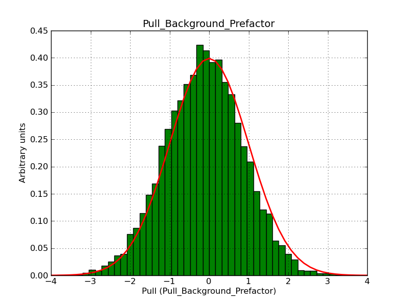 |
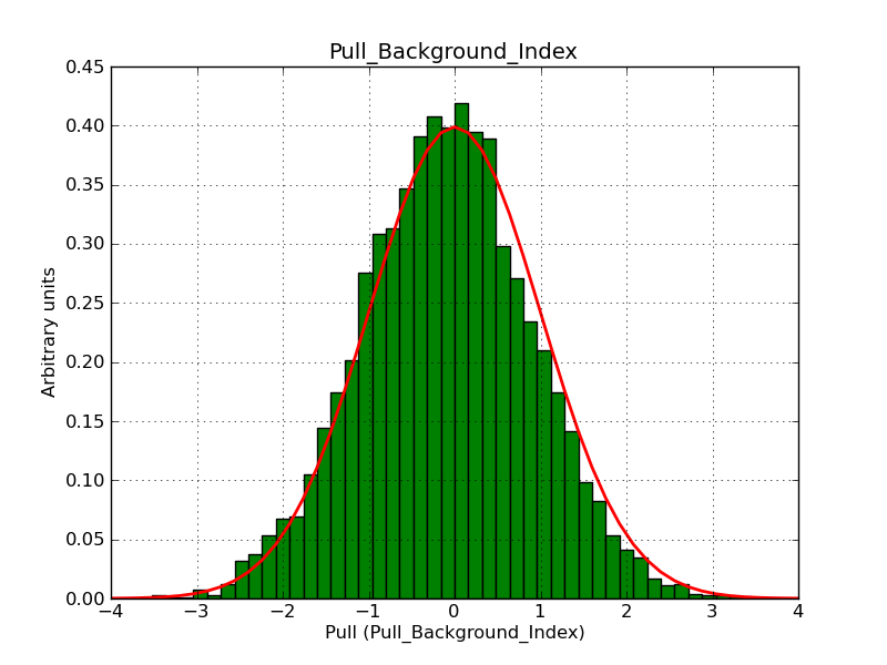 |
| Shell | ||||
| Elliptical Disk |  |
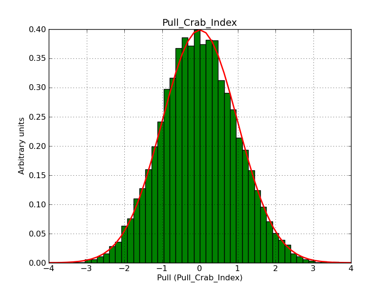 |
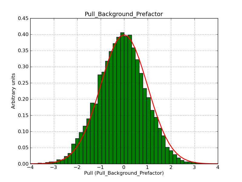 |
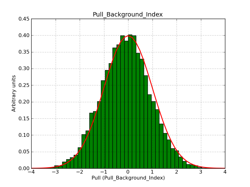 |
| Elliptical Gaussian | ||||
| Map | 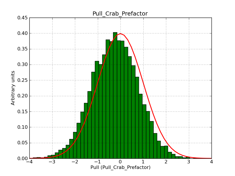 |
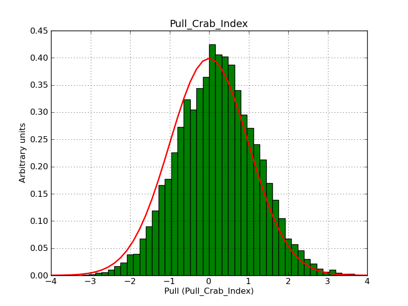 |
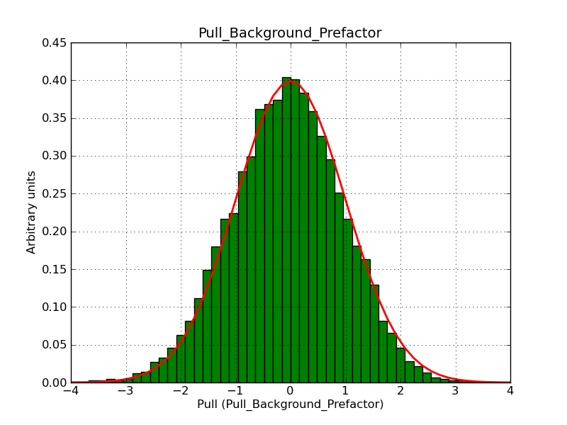 |
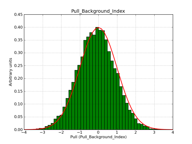 |
Updated over 8 years ago by
The following plots summarize the pull distributions for the spectral models obtained using a stacked analysis.
| Model | Bins | ||||
| Power law | 30 | 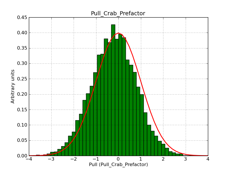 |
 |
||
| Power law 2 | 30 | 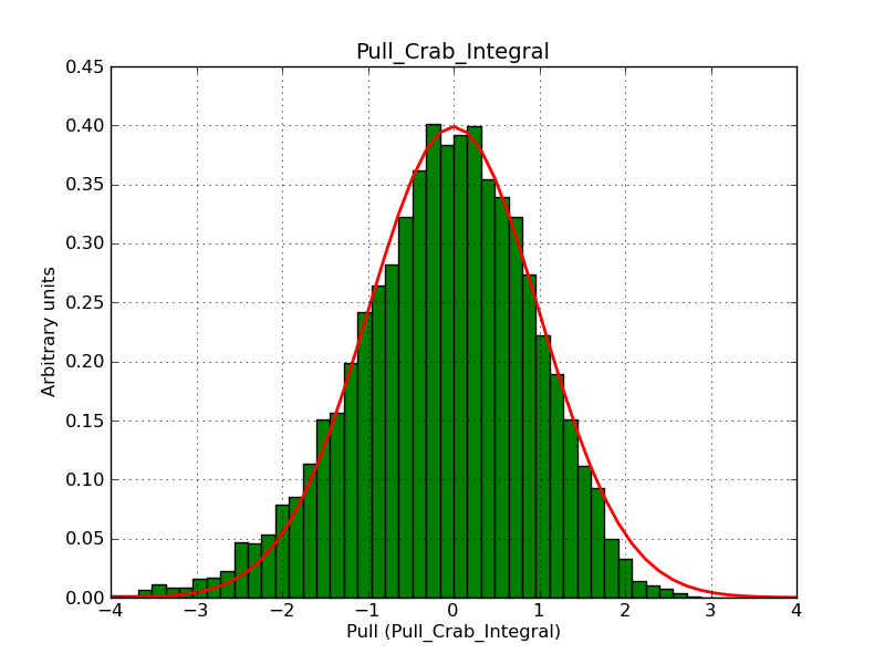 |
 |
||
| Broken power law | 30 | 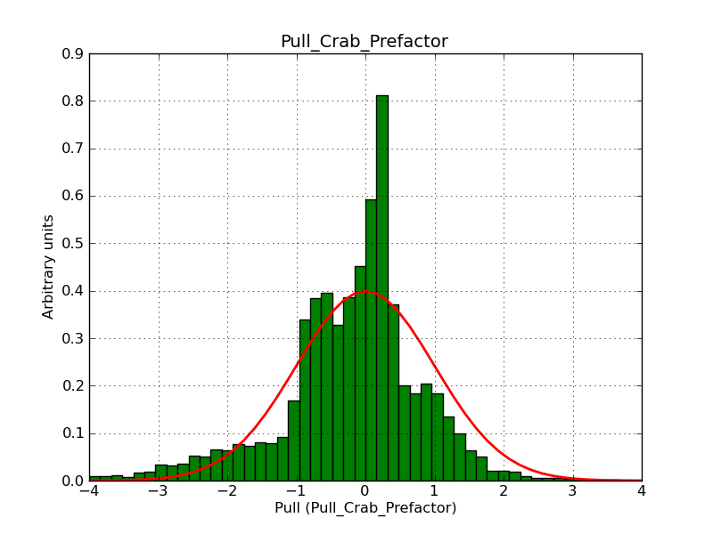 |
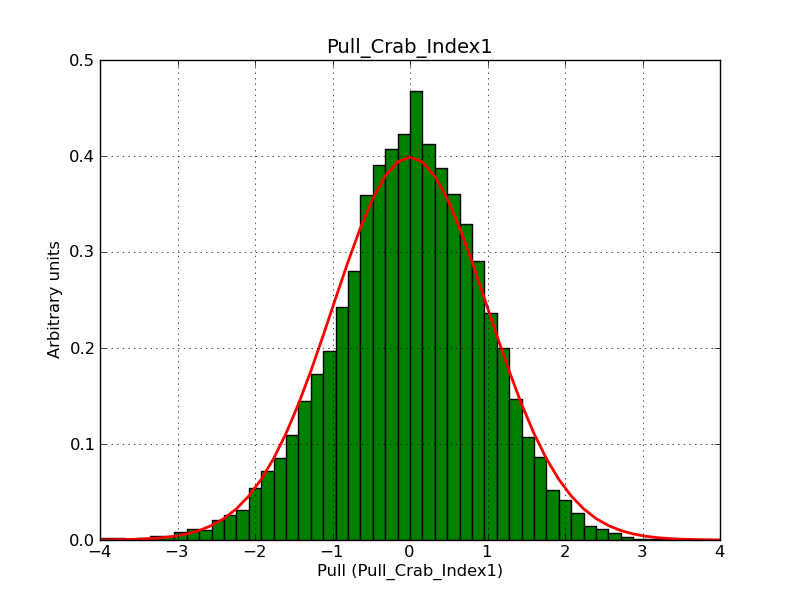 |
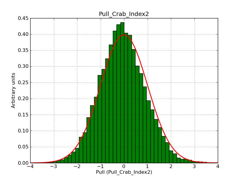 |
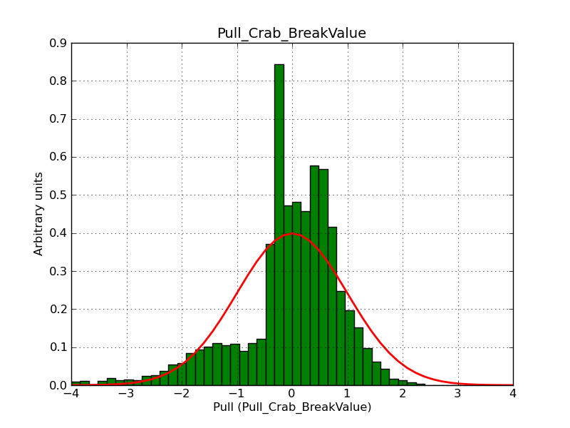 |
| Exponential cut-off power law | 30 | 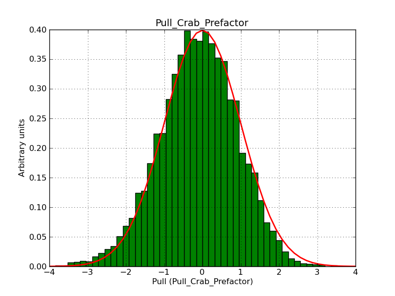 |
 |
 |
|
| Super exponential cut-off power law | 30 | 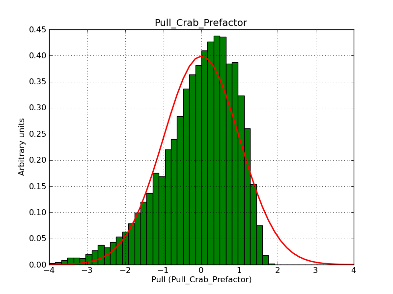 |
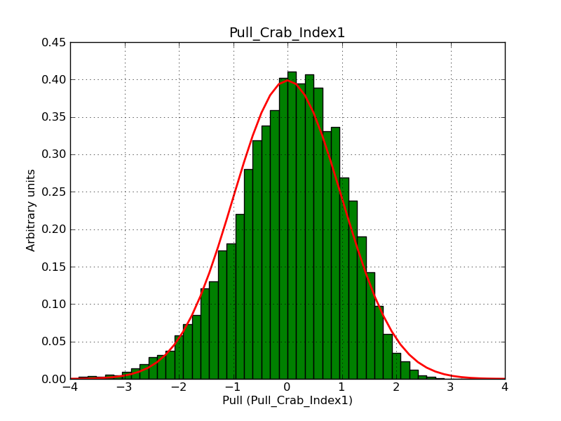 |
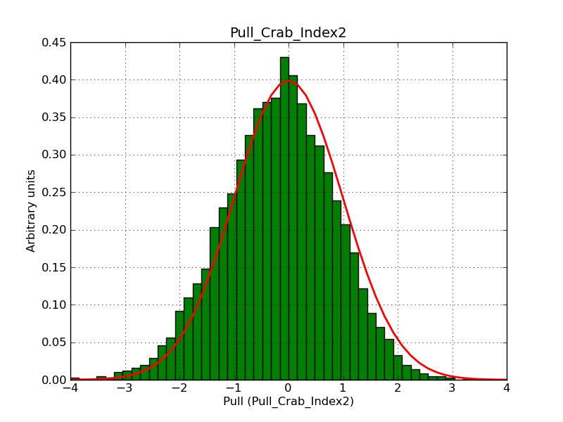 |
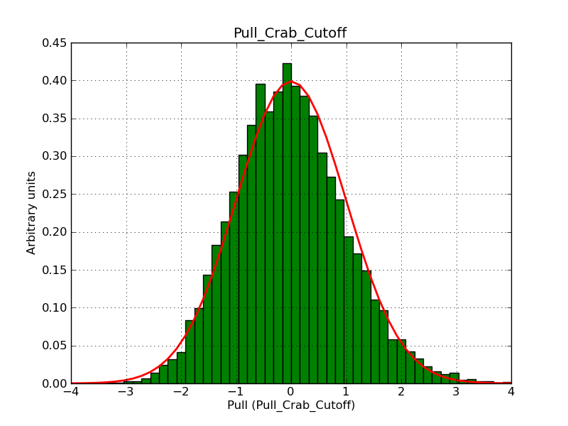 |
| Log parabola | 60 | 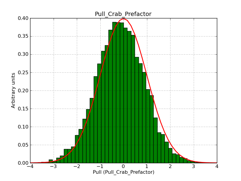 |
 |
 |
|
| File function | 30 | 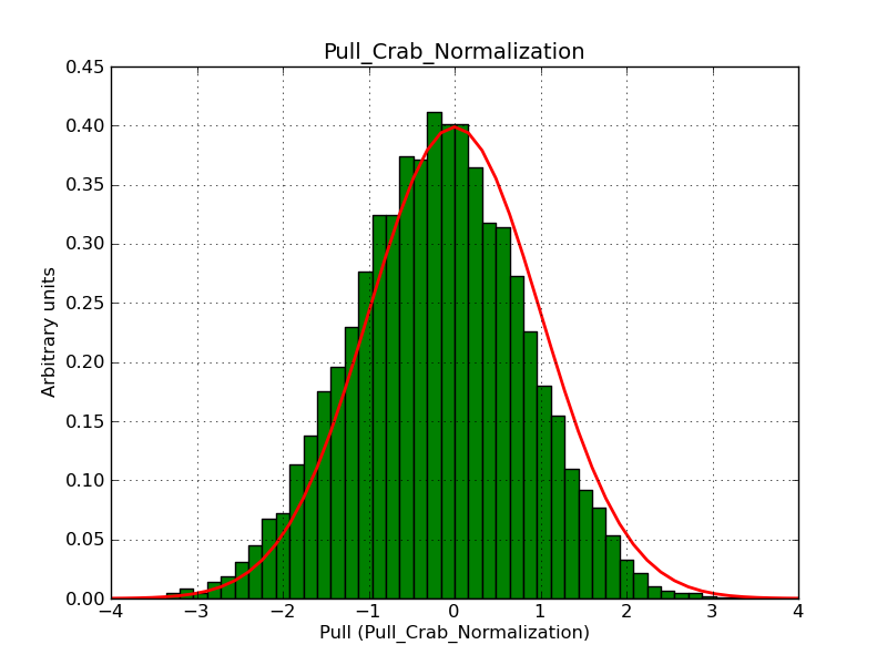 |
|||
| Node function | 30 | 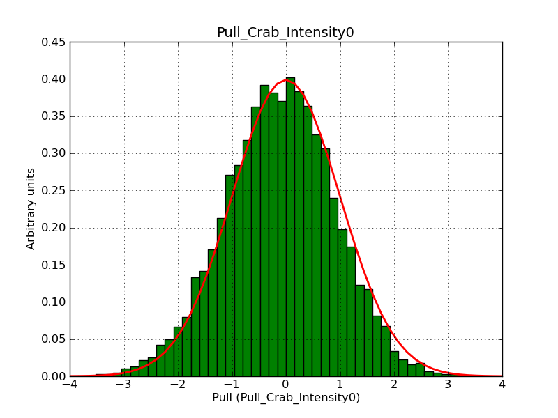 |
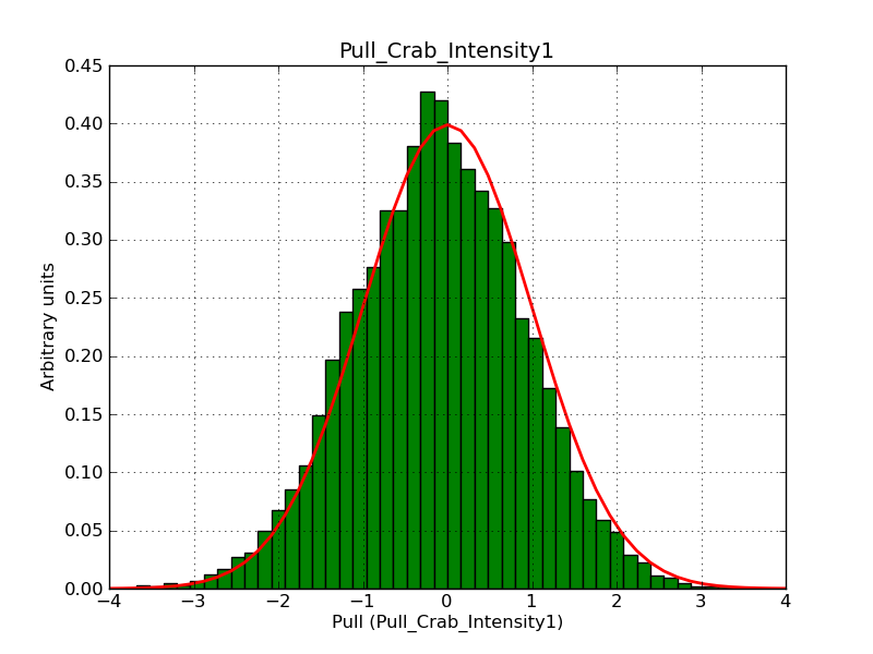 |
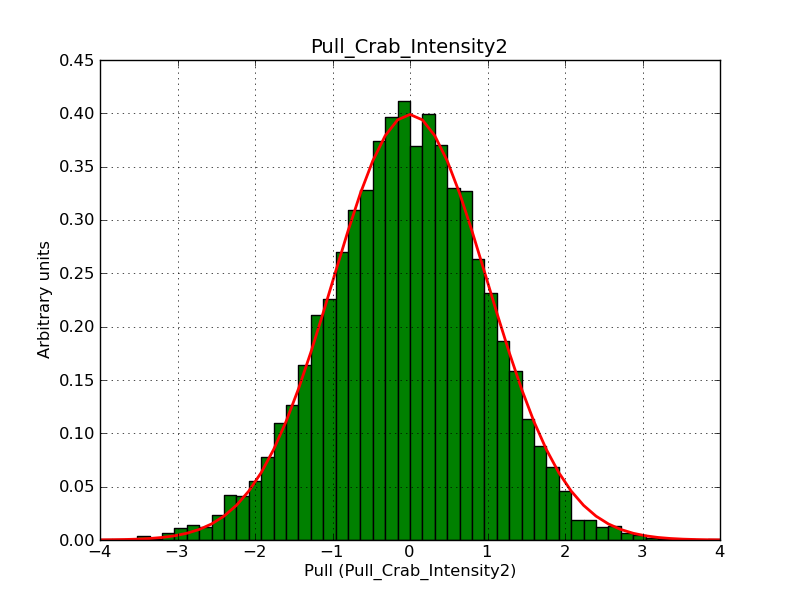 |
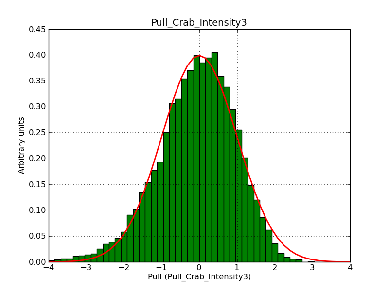 |
| Gauss | 30 |  |
 |
 |
Updated over 8 years ago by
This section summarized pull distributions for spectral laws using unbinned analysis. The model has been fitted on top of the background model. Only the spectral parameters shown have been left free in the spectral fit.
| Model | |||||
| Power law |  |
 |
|||
| Power law 2 | 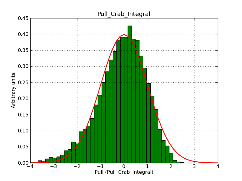 |
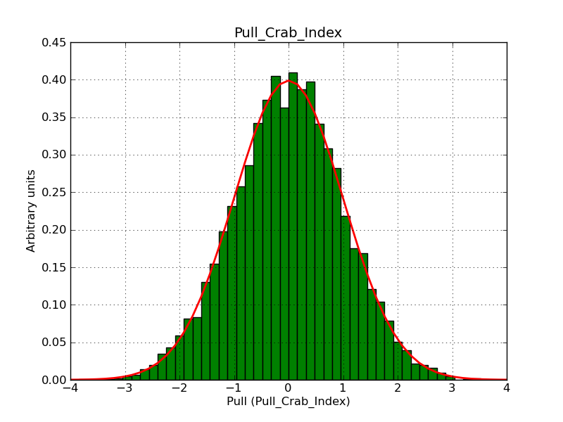 |
|||
| Broken power law | 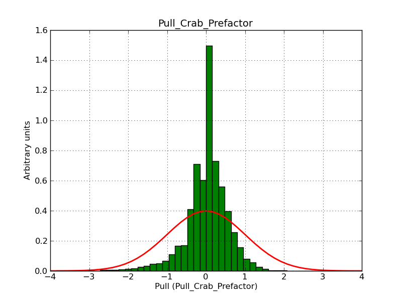 |
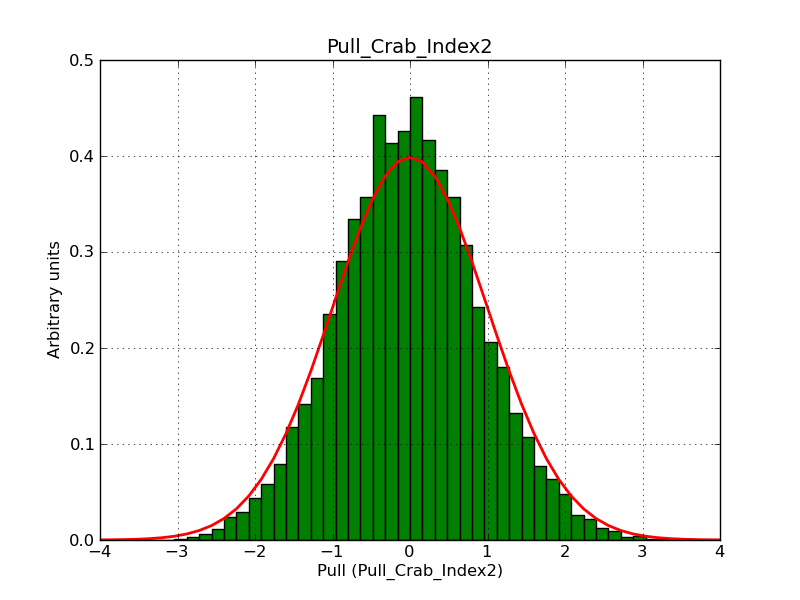 |
|
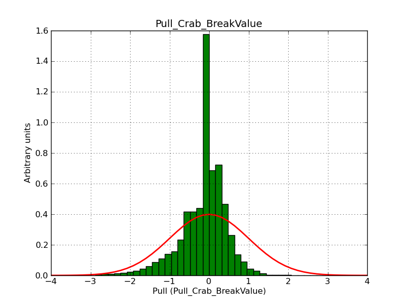 |
|
| Exponentially cut off power law (1800 sec) | 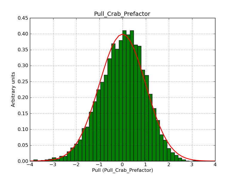 |
 |
 |
||
| Exponentially cut off power law (18000 sec) |  |
 |
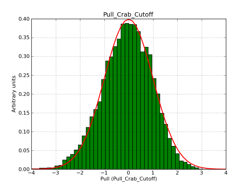 |
||
| Super exponentially cut off power law (1800 sec) | 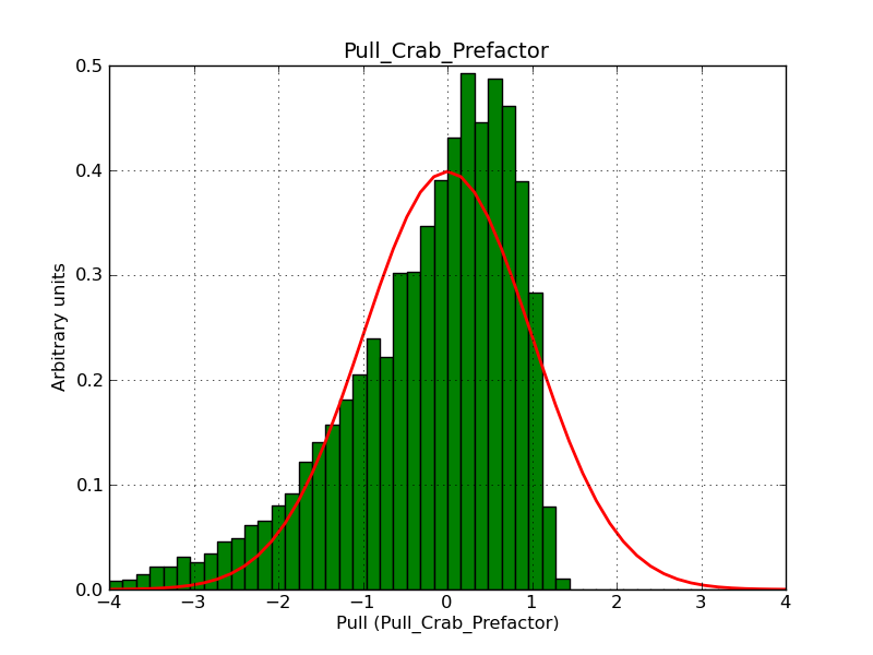 |
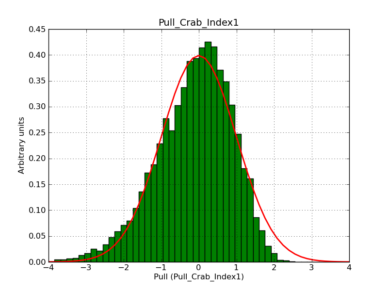 |
 |
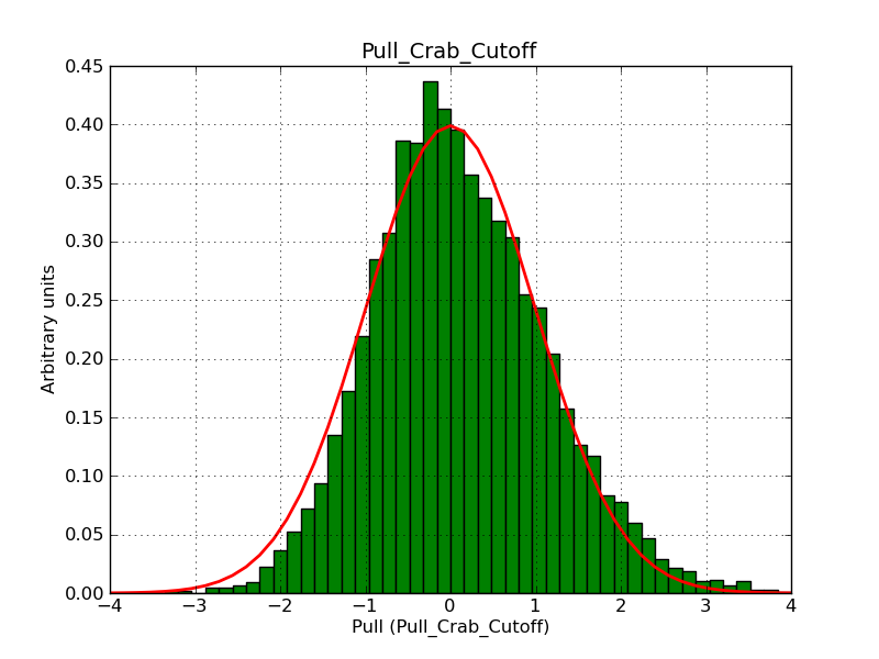 |
|
| Super exponentially cut off power law (18000 sec) | 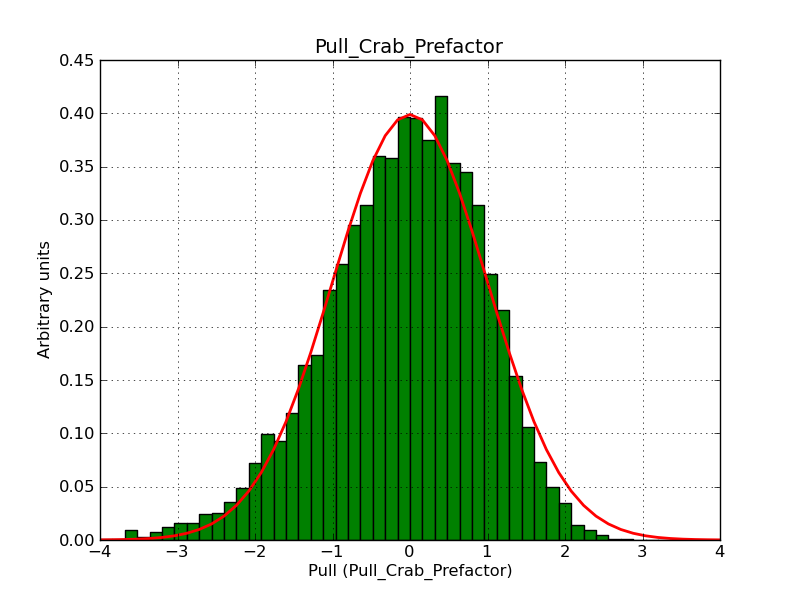 |
 |
 |
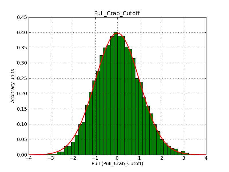 |
|
| Log parabola | 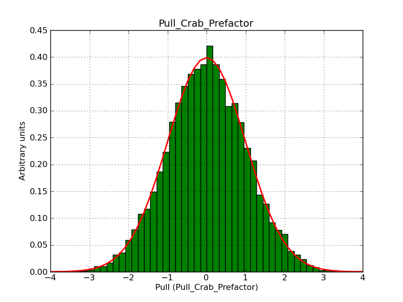 |
 |
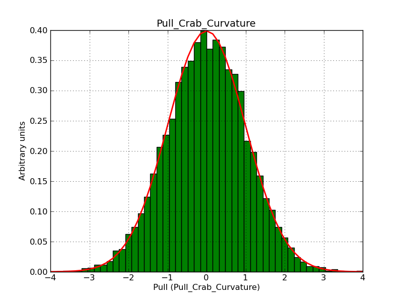 |
||
| File function |  |
||||
| Node function | 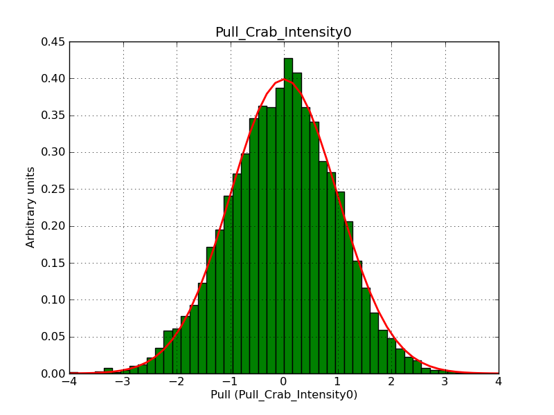 |
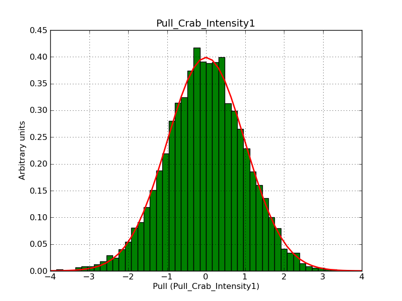 |
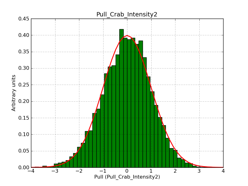 |
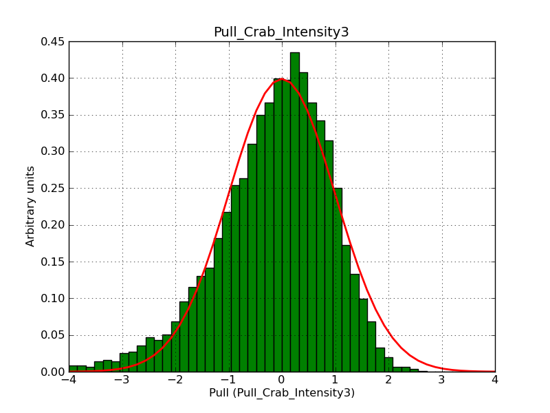 |
|
| Gauss |  |
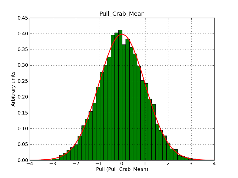 |
 |
Updated almost 12 years ago by
This pages summarizes the work done during the summer project of Jean-Bapsiste Cayrou.
http://franckh.developpez.com/tutoriels/posix/pthreads/
http://www.scsc.no/blog/2010/09-03-creating-pthreads-in-c++-using-pointers-to-member-functions.html
http://jessenoller.com/2009/02/01/python-threads-and-the-global-interpreter-lock/
(just to recall that the GIL exists, but if we use the UNIX pthread mechanism we may be able to circumvent this).
http://openmp.org/mp-documents/ntu-vanderpas.pdf
http://software.intel.com/en-us/articles/getting-started-with-openmp/
Updated almost 12 years ago by
Submissions should be written in english.
Before submitting a bug notification, please check the list of bugs to see whether your bug is already known. If yes, you may add some information to the known bug using the Update tag.
If the bug is not yet known, please create a new issue using the Bug tracker by specifyingPlease do not assign any priority or person, due date and estimated time, this will be handled by the project manager. You may add files as necessary (e.g. configuration file and output, log files, screen dumps, etc.).
Before submitting a feature request, please check the list of feature requests to see whether your feature request is already filed. If yes, you may add some information to the feature request using the Update tag.
If the feature is not yet files, please create a new issue using the Feature tracker by specifyingPlease do not assign any priority or person, due date and estimated time, this will be handled by the project manager. You may add files as necessary (e.g. configuration file and output, log files, screen dumps, etc.).
When you edit a wiki page to improve its content, make sure that you fill the comment field with a descriptive summary of the changes you’ve made to the page. This way we’ll be better able to “monitor” and “maintain” the quality of the actual wiki content.
If you would like to contribute to the GammaLib development, please contact jurgen.knodlseder@irap.omp.eu.
Updated over 2 years ago by
The TRA file format is used by MEGALib to store event information. Check the MEGALib methods src/revan/src/MRERawEvent::ParseLine to better understand how to interpret the format. Note the inheritance of this class:
class MRERawEvent : public MRESE, public MRotationInterface
1970-01-01T01:00:00.Here is the relevant code in src/revan/src/MRERawEvent::ParseLine:
m_EventTime.Set(Line)
bool MTime::Set(const char* Line)
m_Seconds
m_NanoSeconds
}
TI=1465776080.278382500 that gives the event time in UTC:time = gammalib.GTime('1970-01-01T01:00:00')
time += 1465776080.278382500
print(time.utc())
2016-06-13T01:00:54
m_DetectorRotationXAxis[0] [cm] (default: 1.0)m_DetectorRotationXAxis[1] [cm] (default: 0.0)m_DetectorRotationXAxis[2] [cm] (default: 0.0)m_DetectorRotationZAxis[0] [cm] (default: 0.0)m_DetectorRotationZAxis[1] [cm] (default: 0.0)m_DetectorRotationZAxis[2] [cm] (default: 1.0)Longitude [deg]Latitude [deg]SetGalacticPointingXAxis(Longitude, Latitude)
Longitude [deg]Latitude [deg]SetGalacticPointingZAxis(Longitude, Latitude)
Azimuth [deg]Altitude [deg]The information is set by
m_HorizonPointingXAxis.SetMagThetaPhi(1.0, (90-Altitude)*c_Rad, Azimuth*c_Rad)
MVector::SetMagThetaPhi methodvoid MVector::SetMagThetaPhi(double Magnitude, double Theta, double Phi)
{
// Set in spherical coordinates
double A = fabs(Magnitude);
m_X = A*sin(Theta)*cos(Phi);
m_Y = A*sin(Theta)*sin(Phi);
m_Z = A*cos(Theta);
}
Azimuth [deg]Altitude [deg]The same method
m_HorizonPointingZAxis.SetMagThetaPhi(1.0, (90-Altitude)*c_Rad, Azimuth*c_Rad)
MComptonEvent class.m_Eg [keV]m_dEg [keV]m_Ee [keV]m_dEe [keV]MComptonEvent class.m_C1[0] [cm]m_C1[1] [cm]m_C1[2] [dm]m_dC1[0] [cm]m_dC1[1] [cm]m_dC1[2] [dm]m_C2[0] [cm]m_C2[1] [cm]m_C2[2] [dm]m_dC2[0] [cm]m_dC2[1] [cm]m_dC2[2] [dm]m_Ce[0] [cm]m_Ce[1] [cm]m_Ce[2] [dm]m_dCe[0] [cm]m_dCe[1] [cm]m_dCe[2] [dm]MComptonEvent class.m_TrackLength [cm]MComptonEvent class.m_TrackInitialDeposit [keV]MComptonEvent class.m_LeverArm [cm]MComptonEvent class.m_SequenceLengthMComptonEvent class.m_ClusteringQualityFactorMComptonEvent class.m_ComptonQualityFactor1m_ComptonQualityFactor2 (optional, default: 1.0)In the detector system, the event scatter direction is defined by Chi and Psi, where Chi is an azimuth angle and Psi is a zenith angle. The computation of Chi and Psi is done in MEGAlib in src/response/src/MResponseImagingBinnedMode::Analyze:
  // Get the data space information
  MRotation Rotation = Compton->GetDetectorRotationMatrix();

  double Phi = Compton->Phi()*c_Deg;
  MVector Dg = -Compton->Dg();
  Dg = Rotation*Dg;
  double Chi = Dg.Phi()*c_Deg;
  while (Chi < -180) Chi += 360.0;
  while (Chi > +180) Chi -= 360.0;
  double Psi = Dg.Theta()*c_Deg;
  // Direction of the second gamma-ray:
  m_Dg = (m_C2 - m_C1).Unit();
src/misc/src/MComptonEvent::Validate.
The Compton scatter angle is computed in MEGAlib in src/global/misc/src/MComptonEvent::CalculatePhi
bool MComptonEvent::CalculatePhi()
{
  // Compute the compton scatter angle due to the standard equation
  // i.e neglect the movement of the electron,
  // which would lead to a Doppler-broadening
  //
  // Attention, make sure to test before you call this method,
  //            that the Compton-kinematics is correct

  double Value = 1 - c_E0 * (1/m_Eg - 1/(m_Ee + m_Eg));

  if (Value <= -1 || Value >= 1) {
    return false;
  }

  m_Phi = acos(Value);

  return true;
}
In MEGAlib, an intersection test with the Earth horizon is done in src/mimrec/src/MEarthHorizon::IsEventFromEarthByIntersectionTest
bool MEarthHorizon::IsEventFromEarthByIntersectionTest(MPhysicalEvent* Event, bool DumpOutput) const
{
  if (Event->GetType() == MPhysicalEvent::c_Compton) {
    MComptonEvent* C = dynamic_cast<MComptonEvent*>(Event);

    double Phi = C->Phi();

    MVector ConeAxis = -C->Dg();

    // Rotate the ConeAxis into the Earth system:
    ConeAxis = C->GetHorizonPointingRotationMatrix()*ConeAxis;

    // Distance between the Earth cone axis and the Compton cone axis:
    double AxisDist = m_PositionEarth.Angle(ConeAxis);

    if (fabs(AxisDist - Phi) > m_HorizonAngle) {
      return false;
    } else {
      if (DumpOutput == true) {
        mout<<"ID "<<Event->GetId()<<": Cone intersects Earth: "<<AxisDist + Phi<<" < "<<m_HorizonAngle<<endl;
      }
      return true;
    }
  } else if (Event->GetType() == MPhysicalEvent::c_Pair) {
    MPairEvent* P = dynamic_cast<MPairEvent*>(Event);
    double AxisDist = m_PositionEarth.Angle(P->GetOrigin());

    if (AxisDist < m_HorizonAngle) {
      if (DumpOutput == true) {
        mout<<"ID "<<Event->GetId()<<": Origin inside Earth: "<<AxisDist<<" < "<<m_HorizonAngle<<endl;
      }
      return true;
    }
  }

  return false;
}
MRotation MRotationInterface::GetHorizonPointingRotationMatrix() const
{
  // Return the rotation matrix of this event

  // Verify that x and z axis are at right angle:
  if (fabs(m_HorizonPointingXAxis.Angle(m_HorizonPointingZAxis) - c_Pi/2.0)*c_Deg > 0.1) {
    cout<<"Event "<<m_Id<<": Horizon axes are not at right angle, but: "<<m_HorizonPointingXAxis.Angle(m_HorizonPointingZAxis)*c_Deg<<" deg"<<endl;
  }

  // First compute the y-Axis vector:
  MVector m_HorizonPointingYAxis = m_HorizonPointingZAxis.Cross(m_HorizonPointingXAxis);

  return MRotation(m_HorizonPointingXAxis.X(), m_HorizonPointingYAxis.X(), m_HorizonPointingZAxis.X(),
                   m_HorizonPointingXAxis.Y(), m_HorizonPointingYAxis.Y(), m_HorizonPointingZAxis.Y(),
                   m_HorizonPointingXAxis.Z(), m_HorizonPointingYAxis.Z(), m_HorizonPointingZAxis.Z());
}
double MVector::Angle(const MVector& V) const
{
  // Calculate the angle between two vectors:
  // cos Angle = (v dot w) / (|v| x |w|)

  // Protect against division by zero:
  double Denom = Mag()*V.Mag();
  if (Denom == 0) {
    return 0.0;
  } else {
    double Value = Dot(V)/Denom;
    if (Value >  1.0) Value =  1.0;
    if (Value < -1.0) Value = -1.0;
    return acos(Value);
  }
}
m_PositionEarth = MVector(0, 0, -1);
m_HorizonAngle = 90*c_Rad;
MEarthHorizon constructor). The values are set usingbool MEarthHorizon::SetEarthHorizon(const MVector& PositionEarth,
const double HorizonAngle)
{
m_PositionEarth = PositionEarth.Unit();
m_HorizonAngle = HorizonAngle;
return true;
}
src/mimrec/src/MEventSelector.cxx.
Alternatively, a probabilistic evaluation is done using
bool MEarthHorizon::IsEventFromEarthByProbabilityTest(MPhysicalEvent* Event, bool DumpOutput) const
{
  massert(Event != 0);

  if (Event->GetType() == MPhysicalEvent::c_Compton) {
    MComptonEvent* C = dynamic_cast<MComptonEvent*>(Event);

    // Take care of scatter angles larger than 90 deg:
    double Phi = C->Phi();
    MVector ConeAxis = C->Dg();
    // Rotate the ConeAxis into the Earth system:
    ConeAxis = C->GetHorizonPointingRotationMatrix()*ConeAxis;

    MVector Origin = C->DiOnCone();

    // That's the trick, but I don't remember what it means...
    if (Phi > c_Pi/2.0) {
      Phi = c_Pi - Phi;
    } else {
      ConeAxis *= -1;
    }

    // Distance between the Earth cone axis and the Compton cone axis:
    double EarthConeaxisDist = m_PositionEarth.Angle(ConeAxis);

    // Now determine both angles between the cone and Earth (simpler now since phi always <= 90)
    // First the one towards the Earth -- if it is smaller than 0 just use fabs
    double AngleEarthCone1 = EarthConeaxisDist - Phi;
    if (AngleEarthCone1 < 0) AngleEarthCone1 = fabs(AngleEarthCone1); // please don't simplify
    // Then the one away from Earth -- if it is > 180 deg then use the smaller angle
    double AngleEarthCone2 = EarthConeaxisDist + Phi;
    if (AngleEarthCone2 > c_Pi) AngleEarthCone2 -= 2*(AngleEarthCone2 - c_Pi);

    // Case a: Cone is completely inside Earth
    if (AngleEarthCone1 < m_HorizonAngle && AngleEarthCone2 < m_HorizonAngle) {
      mdebug<<"EHC: Cone is completely inside Earth"<<endl;
      if (m_MaxProbability < 1.0) {
        if (DumpOutput == true) {
          mout<<"ID "<<Event->GetId()<<": Cone inside Earth"<<endl;
        }
        return true;
      } else {
        // If the probability is 1.0, we are OK with events from Earth
        return false;
      }
    }
    // Case b: Cone is completely outside Earth
    else if (AngleEarthCone1 > m_HorizonAngle && AngleEarthCone2 > m_HorizonAngle) {
      mdebug<<"EHC: Cone is completely outside Earth"<<endl;
      return false;
    }
    // Case c: Cone intersects horizon
    else {
      // Determine the intersection points on the Compton cone:
      mdebug<<"EHC: Cone intersects horizon"<<endl;

      if (sin(EarthConeaxisDist) == 0 || sin(Phi) == 0) {
        merr<<"Numerical boundary: Scattered gamma-ray flew in direction of "
            <<"the Earth axis and the Compton scatter angle is identical with "
            <<"horizon angle (horizon angle="<<m_HorizonAngle*c_Deg
            <<", Earth-coneaxis-distance="<<EarthConeaxisDist*c_Deg
            <<") - or we have a Compton backscattering (180 deg) "
            <<"or no scattering at all (phi="<<Phi*c_Deg<<")... "
            <<"Nevertheless, I am not rejecting event "<<Event->GetId()<<show;
        return false;
      }
      // Law of cosines for the sides of spherical triangles
      double EarthConeaxisIntersectionAngle =
        acos((cos(m_HorizonAngle)-cos(EarthConeaxisDist)*cos(Phi))/(sin(EarthConeaxisDist)*sin(Phi)));

      if (C->HasTrack() == true && m_ValidComptonResponse == true) {
        // Now we have to determine the distance to the origin on the cone:

        double ConeaxisOriginDist = ConeAxis.Angle(Origin);
        double EarthOriginDist = m_PositionEarth.Angle(Origin);

        if (sin(ConeaxisOriginDist) == 0) {
          merr<<"Numerical boundary: The photon's origin is identical with the cone axis...!"
              <<" Nevertheless, I am not rejecting this event "<<Event->GetId()<<show;
          return false;
        }

        // Law of cosines for the sides of spherical triangles
        double EarthConeaxisOriginAngle =
          acos((cos(EarthOriginDist) - cos(EarthConeaxisDist)*cos(ConeaxisOriginDist))/
               (sin(EarthConeaxisDist)*sin(ConeaxisOriginDist)));

        // The intersections on the cone are at EarthConeaxisOriginAngle +-EarthConeaxisIntersectionAngle
        // Let's figure out the probabilities:

        double Probability = 0;

        // Case A: "Maximum" on cone (not necessarily origin) is from *within* Earth:
        if (EarthOriginDist < m_HorizonAngle) {
          // If the intersection are in different Origin-Coneaxis-Hemispheres:
          if (EarthConeaxisOriginAngle + EarthConeaxisIntersectionAngle < c_Pi) {
            Probability = m_ComptonResponse.GetInterpolated((EarthConeaxisIntersectionAngle - EarthConeaxisOriginAngle)*c_Deg, C->Ee()) +
              m_ComptonResponse.GetInterpolated((EarthConeaxisIntersectionAngle + EarthConeaxisOriginAngle)*c_Deg, C->Ee());
            Probability = 0.5*Probability;

            massert(EarthConeaxisIntersectionAngle - EarthConeaxisOriginAngle >= 0);
            massert(EarthConeaxisIntersectionAngle - EarthConeaxisOriginAngle <= c_Pi);
            massert(EarthConeaxisIntersectionAngle + EarthConeaxisOriginAngle >= 0);
            massert(EarthConeaxisIntersectionAngle + EarthConeaxisOriginAngle <= c_Pi);

          }
          // otherwise:
          else {
            Probability = m_ComptonResponse.GetInterpolated((2*c_Pi - EarthConeaxisIntersectionAngle - EarthConeaxisOriginAngle)*c_Deg, C->Ee()) -
              m_ComptonResponse.GetInterpolated((EarthConeaxisIntersectionAngle - EarthConeaxisOriginAngle)*c_Deg, C->Ee());
            Probability = 1-0.5*Probability;
          }
        }
        // Case B: "Maximum" on cone (not necessarily origin) is from *outside* Earth:
        else {
          // If the intersection are in different hemispheres Origin-Coneaxis-Hemispheres:
          if (EarthConeaxisOriginAngle + EarthConeaxisIntersectionAngle > c_Pi) {
            Probability = m_ComptonResponse.GetInterpolated((EarthConeaxisOriginAngle - EarthConeaxisIntersectionAngle)*c_Deg, C->Ee()) +
              m_ComptonResponse.GetInterpolated((c_Pi + EarthConeaxisIntersectionAngle - EarthConeaxisOriginAngle)*c_Deg, C->Ee());
            Probability = 1-0.5*Probability;
          }
          // otherwise:
          else {
            Probability = m_ComptonResponse.GetInterpolated((EarthConeaxisOriginAngle + EarthConeaxisIntersectionAngle)*c_Deg, C->Ee()) -
              m_ComptonResponse.GetInterpolated((EarthConeaxisOriginAngle - EarthConeaxisIntersectionAngle)*c_Deg, C->Ee());
            Probability = 0.5*Probability;

          }
        }

        if (Probability > m_MaxProbability) {
          if (DumpOutput == true) {
            mout<<"ID "<<Event->GetId()<<": Probability higher max probability: "<<Probability<<" > "<<m_MaxProbability<<endl;
          }
          return true;
        }
      } else {
        // The probability is simply determined by the length of the segment within Earth
        if (EarthConeaxisIntersectionAngle/c_Pi > m_MaxProbability) {
          if (DumpOutput == true) {
            mout<<"ID "<<Event->GetId()<<": Probability higher max probability: "<<EarthConeaxisIntersectionAngle/c_Pi<<" > "<<m_MaxProbability<<endl;
          }
          return true;
        }
      }
    }
  } else if (Event->GetType() == MPhysicalEvent::c_Pair) {
    MPairEvent* P = dynamic_cast<MPairEvent*>(Event);
    double AxisDist = m_PositionEarth.Angle(P->GetOrigin());

    if (AxisDist < m_HorizonAngle) {
      if (DumpOutput == true) {
        mout<<"ID "<<Event->GetId()<<": Origin inside Earth: "<<AxisDist<<" < "<<m_HorizonAngle<<endl;
      }
      return true;
    }
  }

  return false;
}
The following constants are used in MEGAlib:
const double c_Pi = 3.14159265358979311600;
const double c_TwoPi = 2*c_Pi;
const double c_Sqrt2Pi = 2.506628274631;
const double c_Rad = c_Pi / 180.0;
const double c_Deg = 180.0 / c_Pi;
const double c_SpeedOfLight = 29.9792458E+9; // cm/s
const double c_E0 = 510.999; // keV
const double c_FarAway = 1E20; // cm
const double c_LargestEnergy = 0.999*numeric_limits<float>::max();
const MVector c_NullVector(0.0, 0.0, 0.0);
Updated over 11 years ago by Anonymous
Unit testing is a method by which individual units of source code, sets of one or more computer program modules together with associated control data, usage procedures, and operating procedures, are tested to determine if they are fit for use.
In GammaLib, unit tests verify all classes that are provided by the library. Unit testing is initiated using the
$ make checkcommand. So far, the unit tests are implemented using C++ executable that test the various classes. The C++ code of the test executables can be found in the
test directory. Unit tests either compare the results of an operation against the expected value, or our embedded in try - catch blocks to catch unexpected features. In the JUnit parlance (see below), the first types of tests will produce failures, while the second types to tests will produce errors. So far, no distinction is made between failures and errors.
Many frameworks (such as Jenkins or Sonar) support unit test reports in the JUnit format. Also GammaLib should comply to the JUnit XML format specification, so that GammaLib test results can be analyzed and tracked using standard tools. This means, GammaLib unit tests should output the test results in form of XML files that inform about the numbers of failures and errors that occur for a given series of tests. Such series will be combined in test suites, and test suites will be combined in testsuite containers.
We should thus implement a GTestSuites container that contains GTestSuite class elements. Each C++ executable should be mapped into a GTestSuites container. The tests that are done generally within a given function of the test executable (these are the functions that start with a test name, followed by a number of dots, and end by an ok) should be mapped into the GTestSuite.
The GTestSuites container class will run all tests, gather the information about failures and errors, and produce a test report in XML format (see JUnit XML format specification or Jenkins specification for the format definition). The test suite container will dump the container name to the screen in the actual format, e.g.
*************
* CTA tests *
*************
Screen dumping should be optionally disabled. Maybe the
GLog class can be used for this. If one of the tests failed or had en error, the class destructor should exit with an error so that the error will be reported by make check (TBC).
The GTestSuite class will start a series of tests and collects the test information for these series. It provides this information to the container class upon request. For each successful test it will print a . on the screen, failures will results in a F, errors in a E. If all tests are successful, ok will be added at the end of the test to the dump, in case of a failure, NOK will be added. Those are followed by a linefeed. The output will be as follows:
My test: ....F...FEF....F NOK
Another test: ...... ok
Screen dumping should be optionally disabled.
Each test function will now be a test class that derives from GTestSuite, and each test will be a method of this class. The class can have data members that hold information that is passed from one test to the other. It still has to be figured out how the different test methods will register to the class, so that the class can run them one after the other. One possibility is that the class holds a list of pointers. Here a possible implementation (not tested):
class GTestSuite;

typedef bool (GTestSuite::*testpointer)(void);

class GTestSuite {
public:
    GTestSuite() {}
    ~GTestSuite() {}
    void run(void) {
        std::vector<testpointer>::iterator iter;

        for (iter = m_tests.begin(); iter != m_tests.end(); ++iter) {
            try {
                if ((*this.*(*iter))()) {
                    m_success++;
                }
                else {
                    m_failure++;
                }
            }
            catch(std:exception &e) {
                m_error++;
            }
        }
    }
    std::vector<testpointer> m_tests;
};

class MyTestSuite : GTestSuite {
public:
    MyTestSuite();
    ~MyTestSuite() { }
    bool f1(void) {  std::cout << "Unit test 1" << std::endl; return true; }
    bool f2(void) {  std::cout << "Unit test 2" << std::endl; return false; }
private:
    int                      m_a;
};

void MyTestSuite::MyTestSuite(void)
{
    m_tests.push_back(static_cast<testpointer>(&MyTestSuite::f1));
    m_tests.push_back(static_cast<testpointer>(&MyTestSuite::f2));
}

int main() {
    MyTestSuite tests;
    tests.run();
}
#include<vector>
#include<iostream>

class base;

typedef bool (base::*pointer)(void);

class base {
public:
   base() {}
   ~base() {}
   std::vector<pointer> m_fct;
   void run(void) {
       bool r = (this->*(m_fct[0]))();
   }
};

class derived : public base {
public:
   derived() {}
   ~derived() {}
   bool f1(void) { std::cout << "f1" << std::endl; return true; }
   void set(void) {
       m_fct.push_back(static_cast<pointer>(&derived::f1));
   }
};

int main()
{
   derived d;
   d.set();
   d.run();
   return 0;
}
To write a test suite it is necessary to create a class that derives from GTestSuite. This class is abstract so the method void set(void) should be implemented in the derivated class.
The set method contains initialisation of the members used by the test suite and the configuration of the test functions. You can also set the test suite name in this method.
To add a test function (which must be a method of the class), use add_test(static_cast<pfunction>(&myTestSuite::my_test), " Test name");
Each TestSuite should be appended in a TestSuites container and tests are launched by the run() method.
Here an example :
class TestGMyClass : public TestSuite
{
public:

  testGMyClass() : Testsuite() { return; }
  // A test function
  void my_test(void){
    test_assert(1==0,"Test if 1 ==0", "Message if failure");

    // ... some code

    test_try("A specific test")
    try{
       // Some code to test

       test_try_success();
     }
    catch(exception& e)
    {
       test_try_failure(e);
    }
    return;
  }

  void set(void){

   // Set test suite name
   name("Test suite name");

   // Initialisation members
   m_var=0;

   // Add tests
   add_test(static_cast<pfunction>(&myTestSuite::my_test), " Test name");

private:
  int m_var;

};

int main(){
  // Create a conainer of TestSuite
  TestSuites testsuites("GMyClass"');

  // Create our TestSuite
  TestGMyClass testsuite;

  // Append testsuite to the container
  testsuites.append(testsuite);

  // Run all the test suite
  bool was_successful = testsuites.run();

  //save a report
  testsuites.save("reports/GMyClass.xml");

  // Return 0 or 1 depending the tests result.
  return was_successful ? 0 : 1;
}
Reports are saved in the test/reports repertory.
To be compatible with the make check command, the main should return 0 or 1 depending if tests passed or not.
We can also nest test_try. In the test report the name will appear like this : TestFunctionName:TestTryName1:TestTryName2:TestAssertName
Updated over 11 years ago by
GammaLib uses Git for version control. To contribute to the GammaLib source development, you need Git installed on your machine (which is likely already the case). Before using Git, make sure that your user name and e-mail address is correctly configured. This is best done globally using the commands
$ git config --global user.name "Joe Public"
$ git config --global user.email "joe.public@gmail.com"
Please make sure that you specify your full name as user.name, do not use your abbreviated login name because this makes code modification tracking more cryptic.
The GammaLib source code will be accessed using the https protocol, which makes use of SSL certificates. To disable certificate verification, we recommend to issue the command
$ git config --global http.sslverify "false"
which disables certificate verification globally for your installation.
To clone the GammaLib source code, type
$ git clone https://cta-git.irap.omp.eu/gammalib
This will create a directory called gammalib under the current working directory that will contain the GammaLib source code. Note that the default branch from which you should start for software developments is the devel branch, and the git clone command will automatically clone this branch from the central repository. Make sure that you will never use the master branch to start your software developments, as pushing to the master branch is not permitted. The master branch always contains the code of the last GammaLib release, and serves as seed for hotfixes.
The general policy for adding or modifying source code is the creation of a new branch. Suppose you want to create a new feature for GammaLib. In this case, you would issue the command
$ git checkout -b my_new_feature
to create a new branch called my_new_feature. Now you can develop the code, compile and check. Before a first compilation, you need to create the relevant autotools files. This is done by typing
$ ./autogen.sh
$ ./configure
$ make
$ make check
Suppose that you modified the file src/app/GApplication.cpp in creating your new feature. After testing your modification, you will issue the commands
$ git add src/app/GApplication.cpp
$ git commit -m "I added a very nice feature to GammaLib."
to commit your changes. If you omit the -m "I added a very nice feature to GammaLib." part, a vi editor will open to allow you entering a more comprehensive message. Please make sure that your commit message is as meaningful as possible. Describe any developments and changes in detail, and link to the relevant issue by specifying the issue number in the form #nnn, for example: -m "I added a very nice feature to GammaLib that solves the change request #199."
To merge your changes into the central code repository you have to type the following sequence of commands:
$ git checkout devel
$ git pull
$ git merge my_new_feature
$ git push https://user@cta-git.irap.omp.eu/gammalib
The first command will switch your git repository back to the devel branch into which you should merge your new feature. As second command, you should issue the git pull command to make sure that you have the latest version of the GammaLib code in your repository (in case that somebody else has made some modifications since your initial cloning).
The third command will merge your new feature into the development branch. At this stage you have to resolve any code conflicts that may arise from the merging. After merging, and in particular after resolving any code conflicts, test your new feature comprehensively.
Now you’re ready to issue the forth command that will push your new feature back to the central repository. Here, user is your user name on the CTA collaborative platform at IRAP (the same you used to connect for reading this text). Executing this command will open a window that asks for a password (your password on the CTA collaborative platform at IRAP), and after confirming the password, your change will be pushed to the repository.
Typing your password in the window can be avoided by directly specifying the password in the push command:
$ git push https://user:password@cta-git.irap.omp.eu/gammalib
If you want to avoid typing your user name and password every time you make a push, you can create a file called .netrc under your root directory (i.e. ~/.netrc) with the following content:
machine cta-git.irap.omp.eu
  login <user>
  password <password>
(replace <user> and <password> by your user name and password). Once the .netrc file in place, you may simply type
$ git push
to push you code changes into the repository.
Finally, you may delete the obsolete feature branch by typing
$ git branch -d my_new_feature
A nice GUI for handling the GammaLib Git repository is SmartGit (http://www.syntevo.com/smartgit/index.html). This avoids learning all the various Git commands, but requires of course some understanding about how SmartGit works. SmartGit runs on Windows, Mac OS X and Linux.
To configure SmartGit after installation, select Project->Clone... from the menu and configure the repository as follows:
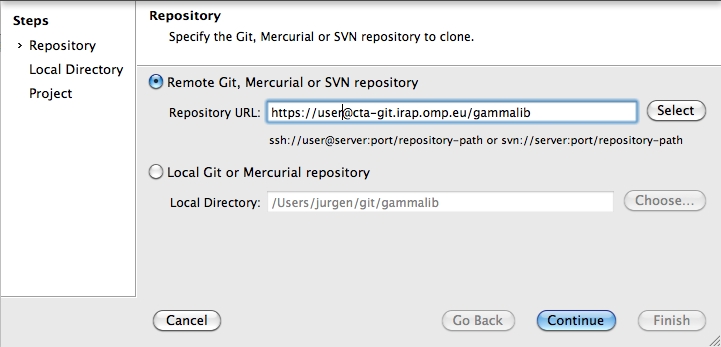
In this example, the user is user. Please replace this field by your own user. After pressing Continue you have to select the repository type:

Press Git here. You will then be asked for you password. If you check the box before Store password, SmartGit will take care of storing your password, and you never have to type it again to interact with the GammaLib Git repository.
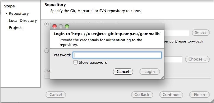
Once logged in you have to specify where the local copy of the Git repository will reside on your disk. Please specify an absolute file path here:
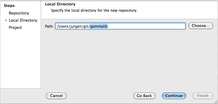
Finally you have to specify a project name and you’re done !

Below a typical view of how the GammaLib repository will be presented by SmartGit (note that the specific directory names and file content will differ in your view):

In case of access problems related to the SSL certificate, make sure you have issued the command
git config --global http.sslverify "false"
in a terminal before. This disables certificate verification globally for your Git installation.
log.txt. You may find this log file in the following directories:
Updated over 11 years ago by
A nice GUI for handling the GammaLib Git repository is SmartGit (http://www.syntevo.com/smartgit/index.html). This avoids learning all the various Git commands, but requires of course some understanding about how SmartGit works. SmartGit runs on Windows, Mac OS X and Linux.
To configure SmartGit after installation, select Project->Clone... from the menu and configure the repository as follows:

In this example, the user is user. Please replace this field by your own user. After pressing Continue you have to select the repository type:
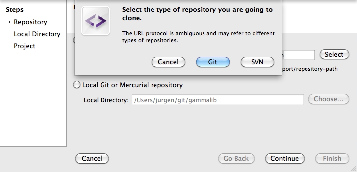
Press Git here. You will then be asked for you password. If you check the box before Store password, SmartGit will take care of storing your password, and you never have to type it again to interact with the GammaLib Git repository.

Once logged in you have to specify where the local copy of the Git repository will reside on your disk. Please specify an absolute file path here:

Finally you have to specify a project name and you’re done !
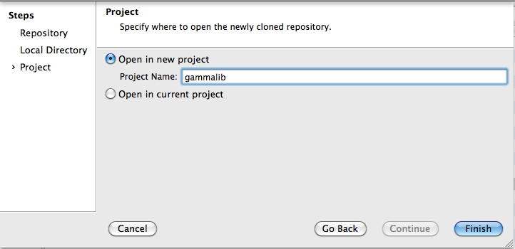
Below a typical view of how the GammaLib repository will be presented by SmartGit (note that the specific directory names and file content will differ in your view):
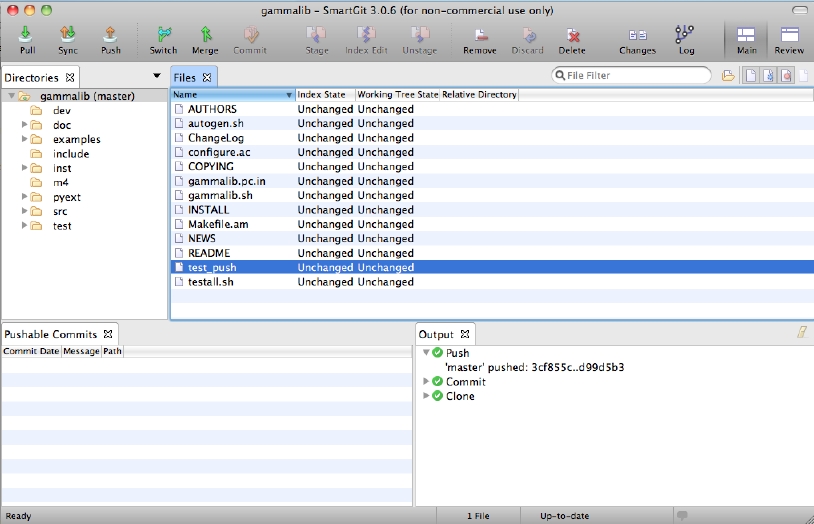
In case of access problems related to the SSL certificate, make sure you have issued the command
$ git config --global http.sslverify "false"in a terminal before. This disables certificate verification globally for your Git installation.
log.txt. You may find this log file in the following directories:
Updated about 10 years ago by Schulz Anneli
The versions of the software are: Science Tools 09-32-05 and ctools (devel from 08.01.14)
Using the following parameters:
ra = 83.6331
dec = 22.0145

rad = 7.5deg,
map: 10x10 deg, 0.1 degperbin
zmax = 100
emin = 100 MeV
emax = 10000 MeV

tmin = 239557446.6 MET in s
tmax= 240162199.6 MET in s
nebins = 20
I performed a standard Fermi analysis and in the end performed a gtlike fit. The data files ( srcmap, exposure cube and ltcube) are produced within the Fermi Science Tools and are the same for gtlike and ctlike.
The model used to describe the data contains only the Crab as a Point Source with a power-law2 spectral model and the galactic and isotropic diffuse models.
| Parameter | gtlike | ctlike |
| Crab integral flux [1e-7] | 25.59 +/- 1.51 | 19.92 +/- 1.19 |
| Crab index | - 2.135 +/- 0.0460 | - 2.051 +/- 0.049 |
| Gal prefac | 0.729 +/- 0.144 | 0.774+/- 0.157 |
| Gal index | 0.087 +/- 0.072 | 0.070 +/- 0.074 |
| Iso normalization | 2.876 +/- 0.686 | 3.486 +/- 0.694 |
The same dataset with the index fixed:
| Parameter | gtlike | ctlike |
| Crab integral flux [1e-7] | 24.87 +/- 1.17 | 20.62 +/- 0.99 |
| Crab index | - 2.1 | - 2.1 |
| Gal prefac | 0.721 +/- 0.145 | 0.783 +/- 0.155 |
| Gal index | 0.085 +/- 0.072 | 0.071 +/- 0.073 |
| Iso normalization | 3.033 +/- 0.657 | 3.326 +/- 0.674 |
the same dataset with the diffuse models fixed:
| Parameter | gtlike | ctlike | |
Crab integral flux [1e-9] | 32.99 +/- 2.29 | 26.35 +/- 1.91 |
| Crab index | - 2.186 +/- 0.041 | - 2.136 +/- 0.042 | ||||
| Gal prefac | 1 | 1 | ||||
| Gal index | 0 | 0 | ||||
| Iso normalization | 1 | 1 | ||||
| nobs | 2225 | 2225 | |
npred | 2193 | 2107.66 |
| log L | 10812 | 10839.8 |
before the fix: 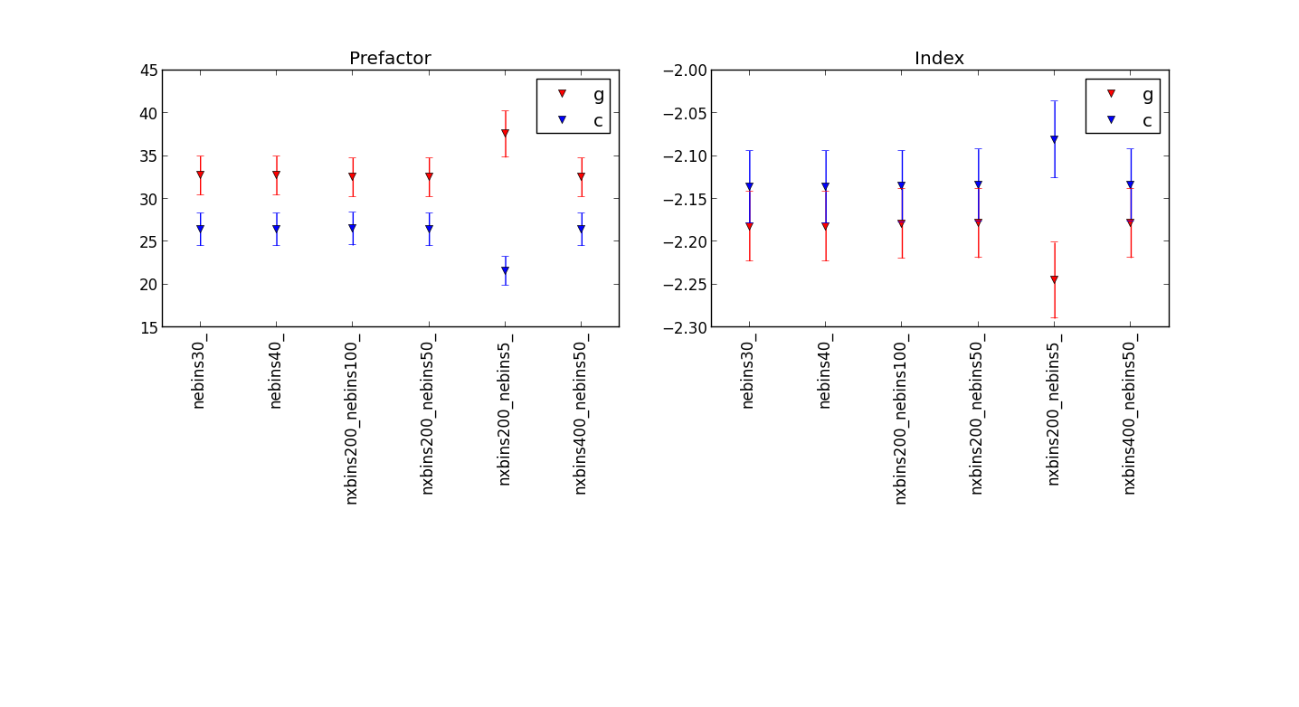
after Jürgen’s fix: 
showing that the fit results are quite similar, but be carful to use enough energy bins.
| Parameter | gtlike | ctlike after fix | ctlike before fix |
| Crab integral flux [1e-7] | 25.59 +/- 1.51 | 25.25 +/- 1.51 | 19.92 +/- 1.19 |
| Crab index | - 2.135 +/- 0.0460 | - 2.137+/- 0.048 | - 2.051 +/- 0.049 |
| Gal prefac | 0.729 +/- 0.144 | 0.728 +/- 0.151 | 0.774+/- 0.157 |
| Gal index | 0.087 +/- 0.072 | 0.078 +/- 0.076 | 0.070 +/- 0.074 |
| Iso normalization | 2.876 +/- 0.686 | 2.912 +/- 0.692 | 3.486 +/- 0.694 |
I also started to investigate the P7REP data/response. For that purpose I create a 20°x20° binned dataset for the first mission week using the P7REP_SOURCE_V15 response. The log file for building the dataset is here: log.txt. The dataset spans 20 logarithmically spaced energy bins from 200 MeV to 20 GeV. I used ScienceTools-09-32-05 and gammalib-00-08-02 / ctools-00-07-02 (10/2/2014).
The gtlike run gives the following results:
<===> Crab:
<===> Integral: 23.7269 +/- 1.75163
<===> Index: -2.13911 +/- 0.05222
<===> LowerLimit: 100
<===> UpperLimit: 500000
<===> TS value: 1420.34
<===> Flux: 1.07194e-06 +/- 5.77353e-08 photons/cm^2/s
<===>
<===> Extragal_diffuse:
<===> Normalization: 1.36172 +/- 0.358261
<===> Flux: 9.47324e-05 +/- 2.49144e-05 photons/cm^2/s
<===>
<===> Galactic_diffuse:
<===> Value: 1.11336 +/- 0.040282
<===> MapBase::readFitsFile: creating WcsMap2 object
<===> Flux: 0.000332391 +/- 1.20257e-05 photons/cm^2/s
<===> WARNING: Fit may be bad in range [3169.79, 3990.52] (MeV)
<===>
<===>
<===> Total number of observed counts: 4832
<===> Total number of model events: 4832.12
<===> 114  -25979.56744  4832.121898
<===>
<===> -log(Likelihood): 25979.56744
The ctlike run gives the following result:
2014-02-10T22:51:21: === GOptimizerLM ===
2014-02-10T22:51:21:  Optimized function value ..: 25988.630
2014-02-10T22:51:21:  Absolute precision ........: 1e-06
2014-02-10T22:51:21:  Optimization status .......: converged
2014-02-10T22:51:21:  Number of parameters ......: 13
2014-02-10T22:51:21:  Number of free parameters .: 4
2014-02-10T22:51:21:  Number of iterations ......: 10
2014-02-10T22:51:21:  Lambda ....................: 1e-13
2014-02-10T22:51:21:  Maximum log likelihood ....: -25988.630
2014-02-10T22:51:21:  Observed events  (Nobs) ...: 4832.000
2014-02-10T22:51:21:  Predicted events (Npred) ..: 4832.000 (Nobs - Npred = 2.56947e-06)
2014-02-10T22:51:21: === GModels ===
2014-02-10T22:51:21:  Number of models ..........: 3
2014-02-10T22:51:21:  Number of parameters ......: 13
2014-02-10T22:51:21: === GModelSky ===
2014-02-10T22:51:21:  Name ......................: Extragal_diffuse
2014-02-10T22:51:21:  Instruments ...............: all
2014-02-10T22:51:21:  Instrument scale factors ..: unity
2014-02-10T22:51:21:  Observation identifiers ...: all
2014-02-10T22:51:21:  Model type ................: DiffuseSource
2014-02-10T22:51:21:  Model components ..........: "ConstantValue" * "FileFunction" * "Constant"
2014-02-10T22:51:21:  Number of parameters ......: 3
2014-02-10T22:51:21:  Number of spatial par's ...: 1
2014-02-10T22:51:21:   Value ....................: 1 [0,10]  (fixed,scale=1,gradient)
2014-02-10T22:51:21:  Number of spectral par's ..: 1
2014-02-10T22:51:21:   Normalization ............: 1.54418 +/- 0.351893 [0,1000]  (free,scale=1,gradient)
2014-02-10T22:51:21:  Number of temporal par's ..: 1
2014-02-10T22:51:21:   Constant .................: 1 (relative value) (fixed,scale=1,gradient)
2014-02-10T22:51:21: === GModelSky ===
2014-02-10T22:51:21:  Name ......................: Galactic_diffuse
2014-02-10T22:51:21:  Instruments ...............: all
2014-02-10T22:51:21:  Instrument scale factors ..: unity
2014-02-10T22:51:21:  Observation identifiers ...: all
2014-02-10T22:51:21:  Model type ................: DiffuseSource
2014-02-10T22:51:21:  Model components ..........: "MapCubeFunction" * "ConstantValue" * "Constant"
2014-02-10T22:51:21:  Number of parameters ......: 3
2014-02-10T22:51:21:  Number of spatial par's ...: 1
2014-02-10T22:51:21:   Normalization ............: 1 [0.001,1000]  (fixed,scale=1,gradient)
2014-02-10T22:51:21:  Number of spectral par's ..: 1
2014-02-10T22:51:21:   Value ....................: 1.09883 +/- 0.0391273 [0,1000]  (free,scale=1,gradient)
2014-02-10T22:51:21:  Number of temporal par's ..: 1
2014-02-10T22:51:21:   Constant .................: 1 (relative value) (fixed,scale=1,gradient)
2014-02-10T22:51:21: === GModelSky ===
2014-02-10T22:51:21:  Name ......................: Crab
2014-02-10T22:51:21:  Instruments ...............: all
2014-02-10T22:51:21:  Instrument scale factors ..: unity
2014-02-10T22:51:21:  Observation identifiers ...: all
2014-02-10T22:51:21:  Model type ................: PointSource
2014-02-10T22:51:21:  Model components ..........: "SkyDirFunction" * "PowerLaw2" * "Constant"
2014-02-10T22:51:21:  Number of parameters ......: 7
2014-02-10T22:51:21:  Number of spatial par's ...: 2
2014-02-10T22:51:21:   RA .......................: 83.6331 [-360,360] deg (fixed,scale=1)
2014-02-10T22:51:21:   DEC ......................: 22.0145 [-90,90] deg (fixed,scale=1)
2014-02-10T22:51:21:  Number of spectral par's ..: 4
2014-02-10T22:51:21:   Integral .................: 2.03031e-06 +/- 1.62742e-07 [1e-14,0.0001] ph/cm2/s (free,scale=1e-07,gradient)
2014-02-10T22:51:21:   Index ....................: -2.09525 +/- 0.06069 [-5,5]  (free,scale=1,gradient)
2014-02-10T22:51:21:   LowerLimit ...............: 100 [10,1e+06] MeV (fixed,scale=1)
2014-02-10T22:51:21:   UpperLimit ...............: 500000 [10,1e+06] MeV (fixed,scale=1)
2014-02-10T22:51:21:  Number of temporal par's ..: 1
2014-02-10T22:51:21:   Constant .................: 1 (relative value) (fixed,scale=1,gradient)
| Parameter | gtlike | ctlike |
| logL | -25979.567 | -25988.630 |
| Fitted counts | 4832.12 | 4832.000 |
| Crab Integral [1e-7] | 23.73 +/- 1.75 | 20.30 +/- 1.63 |
| Crab Index | - 2.14 +/- 0.05 | - 2.10 +/- 0.06 |
| Galactic diffuse | 1.11 +/- 0.04 | 1.10 +/- 0.04 |
| Isotropic | 1.36 +/- 0.36 | 1.54 +/- 0.35 |
The gtlike fit is a little better than the ctlike fit in terms of log likelihood.
The number of counts attributed to the various model components has been determined by running gtlike and ctlike on models containing only the individual model components (for an example, see crab_model.xml; note that gtlike requires some fitting, hence the parameters were free’d within tiny limits around a fixed value). The ctlike run was done using obs_binned.xml. Here the results for the components:
| Component | gtlike logL | gtlike counts | ctlike logL | ctlike counts | gtlike-ctlike counts |
| Crab | -47611.137 | 595.886 | -52867.290 | 586.573 | 9.313 (-1.6%) |
| Isotropic | -35445.565 | 347.113 | -35458.969 | 347.562 | -0.449 (-0.1%) |
| Galactic | -26978.496 | 3380.41 | -26957.335 | 3434.584 | -54.174 (-1.6%) |
| All | -25979.567 | 4832.13 | -25991.482 | 4883.738 | -51.608 (-1.1%) |
The last line shows the results for fitting all components (with parameters held fixed at the optimum gtlike values).
Globally, gtlike and ctlike give within about 2% the same number of counts. Also the likelihoods are comparable (except for the Crab component; the difference is probably related to the different ways of treating zero counts in a model). Hence the response computation looks okay.
The fact that ctlike finds different parameters compared to gtlike seem to relate to a global mix between the model components that is different.
Below a mosaic of model differences for the Crab between Fermi Science Tools and gammalib. The differences are computed for a given source intensity (see crab_model.xml). The Fermi Science Tools model was computed using gtmodel, the gammalib model using lsmodel (a new cscript that I wrote for this purpose, ls means LAT script). gtmodel predicts 595.886 counts, lsmodel 586.573 counts. Images are from first energy bin to last energy (top left to bottom right).
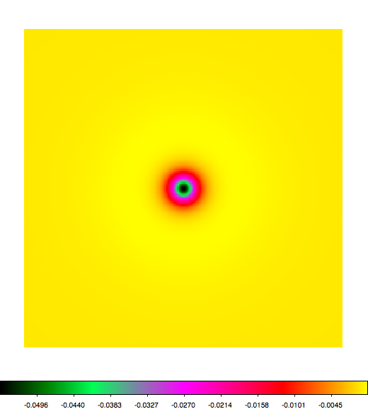 |
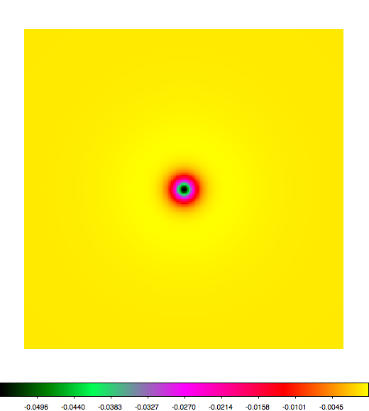 |
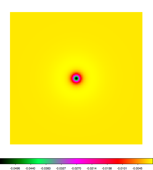 |
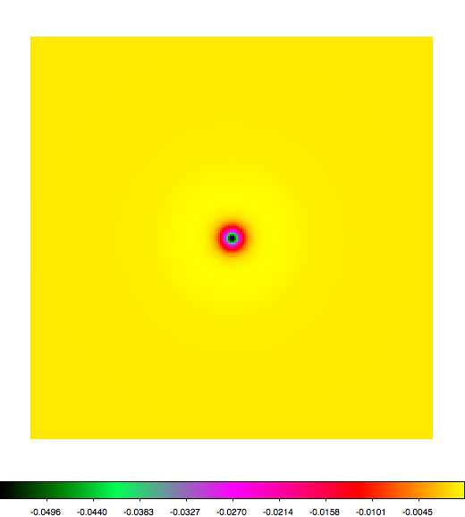 |
 |
 |
 |
 |
 |
 |
 |
 |
 |
 |
 |
 |
 |
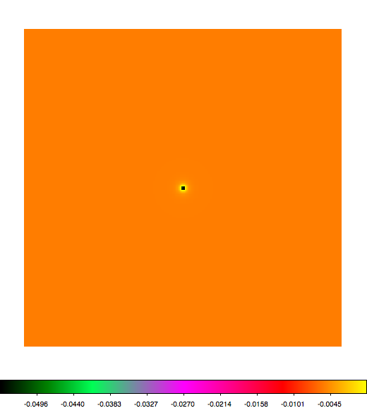 |
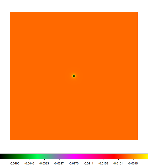 |
 |
A negative residual appears at the position of the Crab, meaning that gammalib predicts more counts at the core of the PSF with respect to the Fermi Science Tools. Conversely, the outer areas in the difference map are positive, indicating that gammalib predicts less counts in the tails of the PSF with respect to the Fermi Science Tools. This picture does not change when each energy bin of the cube is renormalized so that the gammalib and Fermi Science Tools cubes contain the same number of bins. Note that gtmodel has been run using
resample,b,h,yes,,,"Resample input counts map for convolution"
rfactor,i,h,2,,,"Resampling factor"
resample=no is used.
While comparing the ScienceTools to gammalib, I recognised that there was a small difference in the zenith angle range used. GammaLib was constrained to 70° in the GLATMeanPsf class, while in the Fermi/LAT ScienceTools went to the lower boundary of the response array (costheta=0.2). I changed this and verified that both softwares give the same exposure. Below the fit results before and after that change:
| Parameter | gtlike | ctlike before | ctlike after |
| logL | -25979.567 | -25988.630 | -25988.009 |
| Fitted counts | 4832.12 | 4832.000 | 4832.000 |
| Crab Integral [1e-7] | 23.73 +/- 1.75 | 20.30 +/- 1.63 | 20.07 +/- 1.61 |
| Crab Index | - 2.14 +/- 0.05 | - 2.10 +/- 0.06 | - 2.10 +/- 0.06 |
| Galactic diffuse | 1.11 +/- 0.04 | 1.10 +/- 0.04 | 1.10 +/- 0.04 |
| Isotropic | 1.36 +/- 0.36 | 1.54 +/- 0.35 | 1.54 +/- 0.35 |
The impact on the fit results is negligible.
It turned out that the energy scaling of the back response was not correct! In fact, the code used the scaling of the front response for the back response, which resulted in incorrect PSF values for back. After fixing this problem, the following fit results are obtained (“ctlike before” refers to the same values given in the above table, hence before the costheta limit change):
| Parameter | gtlike | ctlike before | ctlike after |
| logL | -25979.567 | -25988.630 | -25980.191 |
| Fitted counts | 4832.12 | 4832.000 | 4832.000 |
| Crab Integral [1e-7] | 23.73 +/- 1.75 | 20.30 +/- 1.63 | 23.56 +/- 1.86 |
| Crab Index | - 2.14 +/- 0.05 | - 2.10 +/- 0.06 | - 2.14 +/- 0.06 |
| Galactic diffuse | 1.11 +/- 0.04 | 1.10 +/- 0.04 | 1.09 +/- 0.04 |
| Isotropic | 1.36 +/- 0.36 | 1.54 +/- 0.35 | 1.44 +/- 0.35 |
This obviously fixed the problem. Now the fit results for the Crab are pretty comparable.
I started working on a larger data set and encountered some differences: one is documented in this issue [[https://cta-redmine.irap.omp.eu/issues/1150]]: , since I first thought that it might be a problem of special spectral models.
I started with an analysis of large dataset (5 years) in a ROI around W49B, which is close to the galactic plane, I have a large number of events:
Observed events (Nobs) ...: 1057409.000
this I fit in science tools ( including the models for 2FGL sources) and get reasonable values for the source and also the diffuse components and the other sources. ( too many numbers to put here)
Now to the cross-check with ctools:
In the beginning I fixed all the sources (except the source of interest) to the fitted values a reanalysed it with ctools.
There the discrepancy between ctools (first value) compared to science tools (second value) is huge:
W49B parameter: norm with value 0.000367931 compared to 0.00605515974 parameter: alpha with value 0.258841 compared to 2.275627162 parameter: beta with value 0.466763 compared to 0.05265050255 parameter: Eb with value 1880.54 compared to 1880.536653
I fixed the Eb to the value from the gtlike fit, since ctools are known to have a problem with correlated parameters (and Eb and norm are in this case). Free Eb makes the result even worse.
The norm of the fitted source is always close to the minimum. So I decided to go for “easier” model and do some checks:
including many sources but fixed to fitted values and only power law, powerlaw2 spectral models.
the second idea was that the reason might be the evaluation of of the PowerLaw with super exponential cutoff or log parabola, since both gave even worse results. But performing several checks I decided to go even a level lower and include only diffuse models in the ctools fit:
The values for the models are ( fitted in gtlike and fixed then in ctlike):
gal: Prefactor ................: 1.06256 [1e-05,100] ph/cm2/s/MeV (fixed,scale=1,gradient) Index ....................: -0.00511337 [-1,1] (fixed,scale=1,gradient) PivotEnergy ..............: 100 [50,2000] MeV (fixed,scale=1,gradient) iso: Normalization ............: 0.356774 [0,10] (fixed,scale=1,gradient)
the number of predicted events in science tools is: 948640 while the number in ctools ( putting the models with fixed values in) is: 958766.087
This discrepancy of 10000 events might lead to wrong fitting results of the sources, which have much lower number of events.
Jürgen:
This is indeed strange. I looked into the srcmap file you sent and found one strange thing: the first and last layer of the isotropic diffuse component look pretty different in comparison to the other layers. For example, the first layer goes from 180174-379102 in value, about a factor 2 in range. The second layer runs from 376238-402911, a much more narrow dynamic range. I won’t expect that the response changes so quickly in energy. The before last layer covers 394973-428132 in range, the last layer covers 336460-409524. So somehow the first and last layers are different. I check with another srcmap file I have a I see not such a strange effect. Can you check the srcmap file and make sure that everything went well in creating the file?
By the way: I note that the predicted events from the ScienceTools (948640) is pretty off the observed number of events (1057409). When I fit the galactic diffuse and isotropic background using ctlike I get exactly the observed number of events and the following fit results:
gal: Prefactor ................: 1.25116 +/- 0.00438167 [1e-05,100] ph/cm2/s/MeV (free,scale=1,gradient) Index ....................: -0.0285025 +/- 0.00138844 [-1,1] (free,scale=1,gradient) PivotEnergy ..............: 100 [50,2000] MeV (fixed,scale=1,gradient) iso: Normalization ............: 0 +/- 0.038531 [0,10] (free,scale=1,gradient)
| Analysis | Norm@300MeV | Index | Curvature |
| ctools | 2.86 ± 0.04 | 1.99 ± 0.13 | 0.06 ± 0.03 |
| FSTs | 2.87 ± 0.02 | 1.98 ± 0.03 | 0.07 ± 0.01 |
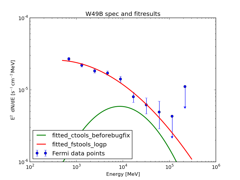
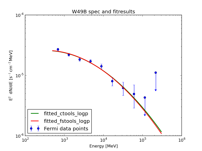
Updated over 11 years ago by
The initial validation of the Pass 7 IRFs has been done using GammaLib-00-06-00. Here the results for several datasets.
| Parameter | gtlike | gammalib (with correction) | gammalib (w/o correction) |
| Counts (for same flux) | 814.987 | 842.551 | 827.99 |
| Flux | 24.23 +/- 1.50 | 19.23 +/- 1.21 | - |
| Spectral index | 2.125 +/- 0.048 | 2.039 +/- 0.051 | - |
| Extragalactic diffuse | 2.286 +/- 0.462 | 2.896 +/- 0.442 | - |
| Galactic diffuse | 0.862 +/- 0.065 | 0.863 +/- 0.064 | - |
Crab: Integral: 24.2369 +/- 1.49572 Index: -2.12467 +/- 0.0476363 LowerLimit: 100 UpperLimit: 500000 TS value: 1300.37 Flux: 2.41076e-06 +/- 1.50551e-07 photons/cm^2/s Total number of model events: 814.987 Extragal_diffuse: Normalization: 2.28565 +/- 0.462091 Flux: 0.000472695 +/- 9.55313e-05 photons/cm^2/s Galactic_diffuse: Value: 0.861504 +/- 0.0652024 Flux: 0.00041505 +/- 3.14108e-05 photons/cm^2/s WARNING: Fit may be bad in range [100, 1258.93] (MeV) WARNING: Fit may be bad in range [1995.26, 5011.87] (MeV) Total number of observed counts: 2211 Total number of model events: 2211 -log(Likelihood): 10794.50987
=== GOptimizerLM === Optimized function value ..: 10814.4 Absolute precision ........: 1e-06 Optimization status .......: converged Number of parameters ......: 13 Number of free parameters .: 4 Number of iterations ......: 9 Lambda ....................: 1e-12 === GObservations === Number of observations ....: 1 Number of predicted events : 2211 === GModels === Number of models ..........: 3 Number of parameters ......: 13 === GModelDiffuseSource === Name ......................: Extragal_diffuse Instruments ...............: all Model type ................: "ConstantValue" * "FileFunction" * "Constant" Number of parameters ......: 3 Number of spatial par's ...: 1 Value ....................: 1 [0,10] (fixed,scale=1,gradient) Number of spectral par's ..: 1 Normalization ............: 2.89602 +/- 0.441842 [0,1000] (free,scale=1,gradient) Number of temporal par's ..: 1 Constant .................: 1 (relative value) (fixed,scale=1,gradient) === GModelDiffuseSource === Name ......................: Galactic_diffuse Instruments ...............: all Model type ................: "MapCubeFunction" * "ConstantValue" * "Constant" Number of parameters ......: 3 Number of spatial par's ...: 1 Normalization ............: 1 [0.001,1000] (fixed,scale=1,gradient) Number of spectral par's ..: 1 Value ....................: 0.862952 +/- 0.0637931 [0,1000] (free,scale=1,gradient) Number of temporal par's ..: 1 Constant .................: 1 (relative value) (fixed,scale=1,gradient) === GModelPointSource === Name ......................: Crab Instruments ...............: all Model type ................: "SkyDirFunction" * "PowerLaw2" * "Constant" Number of parameters ......: 7 Number of spatial par's ...: 2 RA .......................: 83.6331 [-360,360] deg (fixed,scale=1) DEC ......................: 22.0145 [-90,90] deg (fixed,scale=1) Number of spectral par's ..: 4 Integral .................: 1.92253e-06 +/- 1.20962e-07 [1e-14,0.0001] ph/cm2/s (free,scale=1e-07,gradient) Index ....................: -2.03863 +/- 0.0509223 [-5,5] (free,scale=1,gradient) LowerLimit ...............: 100 [10,1e+06] MeV (fixed,scale=1) UpperLimit ...............: 500000 [10,1e+06] MeV (fixed,scale=1) Number of temporal par's ..: 1 Constant .................: 1 (relative value) (fixed,scale=1,gradient)
| Parameter | gtlike | gammalib (with correction) |
| -logL | 2395.656 | 2396.97 |
| Predicted counts | 658.017 | 658 |
| Flux | 26.10 +/- 3.10 | 15.58 +/- 1.95 |
| Spectral index | -2.1 | -2.1 |
| Extragalactic diffuse | 3.47 +/- 1.35 | 3.95 +/- 1.29 |
| Galactic diffuse | 0.68 +/- 0.36 | 0.71 +/- 0.40 |
Crab: Integral: 26.1036 +/- 3.10488 Index: -2.1 LowerLimit: 100 UpperLimit: 500000 TS value: 108.858 Flux: 1.39271e-06 +/- 1.65655e-07 photons/cm^2/s Extragal_diffuse: Normalization: 3.47027 +/- 1.34533 Flux: 0.000427812 +/- 0.000165849 photons/cm^2/s Galactic_diffuse: Value: 0.679862 +/- 0.362457 Flux: 0.000134393 +/- 7.16491e-05 photons/cm^2/s WARNING: Fit may be bad in range [100, 200] (MeV) Total number of observed counts: 658 Total number of model events: 658.017 -log(Likelihood): 2395.656269
2012-07-11T21:55:18: === GOptimizerLM === 2012-07-11T21:55:18: Optimized function value ..: 2396.97 2012-07-11T21:55:18: Absolute precision ........: 1e-06 2012-07-11T21:55:18: Optimization status .......: converged 2012-07-11T21:55:18: Number of parameters ......: 13 2012-07-11T21:55:18: Number of free parameters .: 3 2012-07-11T21:55:18: Number of iterations ......: 6 2012-07-11T21:55:18: Lambda ....................: 1e-09 2012-07-11T21:55:18: Maximum log likelihood ....: -2396.97 2012-07-11T21:55:18: Npred .....................: 658 2012-07-11T21:55:18: === GModels === 2012-07-11T21:55:18: Number of models ..........: 3 2012-07-11T21:55:18: Number of parameters ......: 13 2012-07-11T21:55:18: === GModelDiffuseSource === 2012-07-11T21:55:18: Name ......................: Extragal_diffuse 2012-07-11T21:55:18: Instruments ...............: all 2012-07-11T21:55:18: Model type ................: "ConstantValue" * "FileFunction" * "Constant" 2012-07-11T21:55:18: Number of parameters ......: 3 2012-07-11T21:55:18: Number of spatial par's ...: 1 2012-07-11T21:55:18: Value ....................: 1 [0,10] (fixed,scale=1,gradient) 2012-07-11T21:55:18: Number of spectral par's ..: 1 2012-07-11T21:55:18: Normalization ............: 3.95168 +/- 1.29363 [0,1000] (free,scale=1,gradient) 2012-07-11T21:55:18: Number of temporal par's ..: 1 2012-07-11T21:55:18: Constant .................: 1 (relative value) (fixed,scale=1,gradient) 2012-07-11T21:55:18: === GModelDiffuseSource === 2012-07-11T21:55:18: Name ......................: Galactic_diffuse 2012-07-11T21:55:18: Instruments ...............: all 2012-07-11T21:55:18: Model type ................: "MapCubeFunction" * "ConstantValue" * "Constant" 2012-07-11T21:55:18: Number of parameters ......: 3 2012-07-11T21:55:18: Number of spatial par's ...: 1 2012-07-11T21:55:18: Normalization ............: 1 [0.001,1000] (fixed,scale=1,gradient) 2012-07-11T21:55:18: Number of spectral par's ..: 1 2012-07-11T21:55:18: Value ....................: 0.71251 +/- 0.398651 [0,1000] (free,scale=1,gradient) 2012-07-11T21:55:18: Number of temporal par's ..: 1 2012-07-11T21:55:18: Constant .................: 1 (relative value) (fixed,scale=1,gradient) 2012-07-11T21:55:18: === GModelPointSource === 2012-07-11T21:55:18: Name ......................: Crab 2012-07-11T21:55:18: Instruments ...............: all 2012-07-11T21:55:18: Model type ................: "SkyDirFunction" * "PowerLaw2" * "Constant" 2012-07-11T21:55:18: Number of parameters ......: 7 2012-07-11T21:55:18: Number of spatial par's ...: 2 2012-07-11T21:55:18: RA .......................: 83.6331 [-360,360] deg (fixed,scale=1) 2012-07-11T21:55:18: DEC ......................: 22.0145 [-90,90] deg (fixed,scale=1) 2012-07-11T21:55:18: Number of spectral par's ..: 4 2012-07-11T21:55:18: Integral .................: 1.55815e-06 +/- 1.94647e-07 [1e-14,0.0001] ph/cm2/s (free,scale=1e-07,gradient) 2012-07-11T21:55:18: Index ....................: -2.1 [-5,5] (fixed,scale=1,gradient) 2012-07-11T21:55:18: LowerLimit ...............: 100 [10,1e+06] MeV (fixed,scale=1) 2012-07-11T21:55:18: UpperLimit ...............: 500000 [10,1e+06] MeV (fixed,scale=1) 2012-07-11T21:55:18: Number of temporal par's ..: 1 2012-07-11T21:55:18: Constant .................: 1 (relative value) (fixed,scale=1,gradient)
| Parameter | gtlike | gammalib (with correction) |
| -logL | 874.856 | 879.393 |
| Predicted counts | 213.042 | 213 |
| Flux | 27.72 +/- 3.30 | 25.58 +/- 3.21 |
| Spectral index | -2.1 | -2.1 |
| Extragalactic diffuse | 0.00019418 +/- 0.0433937 | 0 +/- 5.5129 |
| Galactic diffuse | 0.95 +/- 0.09 | 0.85 +/- 0.25 |
Crab: Integral: 27.7185 +/- 3.29829 Index: -2.1 LowerLimit: 100 UpperLimit: 500000 TS value: 335.184 Flux: 1.17471e-07 +/- 1.39781e-08 photons/cm^2/s Extragal_diffuse: Normalization: 0.00019418 +/- 0.0433937 Flux: 7.9062e-10 +/- 1.7668e-07 photons/cm^2/s Galactic_diffuse: Value: 0.952101 +/- 0.092758 Flux: 2.87516e-05 +/- 2.8011e-06 photons/cm^2/s WARNING: Fit may be bad in range [1000, 2000] (MeV) Total number of observed counts: 213 Total number of model events: 213.042 -log(Likelihood): 874.8585611
2012-07-11T22:11:46: === GOptimizerLM === 2012-07-11T22:11:46: Optimized function value ..: 879.393 2012-07-11T22:11:46: Absolute precision ........: 1e-06 2012-07-11T22:11:46: Optimization status .......: converged 2012-07-11T22:11:46: Number of parameters ......: 13 2012-07-11T22:11:46: Number of free parameters .: 3 2012-07-11T22:11:46: Number of iterations ......: 23 2012-07-11T22:11:46: Lambda ....................: 1 2012-07-11T22:11:46: Maximum log likelihood ....: -879.393 2012-07-11T22:11:46: Npred .....................: 213 2012-07-11T22:11:46: === GModels === 2012-07-11T22:11:46: Number of models ..........: 3 2012-07-11T22:11:46: Number of parameters ......: 13 2012-07-11T22:11:46: === GModelDiffuseSource === 2012-07-11T22:11:46: Name ......................: Extragal_diffuse 2012-07-11T22:11:46: Instruments ...............: all 2012-07-11T22:11:46: Model type ................: "ConstantValue" * "FileFunction" * "Constant" 2012-07-11T22:11:46: Number of parameters ......: 3 2012-07-11T22:11:46: Number of spatial par's ...: 1 2012-07-11T22:11:46: Value ....................: 1 [0,10] (fixed,scale=1,gradient) 2012-07-11T22:11:46: Number of spectral par's ..: 1 2012-07-11T22:11:46: Normalization ............: 0 +/- 5.5129 [0,1000] (free,scale=1,gradient) 2012-07-11T22:11:46: Number of temporal par's ..: 1 2012-07-11T22:11:46: Constant .................: 1 (relative value) (fixed,scale=1,gradient) 2012-07-11T22:11:46: === GModelDiffuseSource === 2012-07-11T22:11:46: Name ......................: Galactic_diffuse 2012-07-11T22:11:46: Instruments ...............: all 2012-07-11T22:11:46: Model type ................: "MapCubeFunction" * "ConstantValue" * "Constant" 2012-07-11T22:11:46: Number of parameters ......: 3 2012-07-11T22:11:46: Number of spatial par's ...: 1 2012-07-11T22:11:46: Normalization ............: 1 [0.001,1000] (fixed,scale=1,gradient) 2012-07-11T22:11:46: Number of spectral par's ..: 1 2012-07-11T22:11:46: Value ....................: 0.84716 +/- 0.248145 [0,1000] (free,scale=1,gradient) 2012-07-11T22:11:46: Number of temporal par's ..: 1 2012-07-11T22:11:46: Constant .................: 1 (relative value) (fixed,scale=1,gradient) 2012-07-11T22:11:46: === GModelPointSource === 2012-07-11T22:11:46: Name ......................: Crab 2012-07-11T22:11:46: Instruments ...............: all 2012-07-11T22:11:46: Model type ................: "SkyDirFunction" * "PowerLaw2" * "Constant" 2012-07-11T22:11:46: Number of parameters ......: 7 2012-07-11T22:11:46: Number of spatial par's ...: 2 2012-07-11T22:11:46: RA .......................: 83.6331 [-360,360] deg (fixed,scale=1) 2012-07-11T22:11:46: DEC ......................: 22.0145 [-90,90] deg (fixed,scale=1) 2012-07-11T22:11:46: Number of spectral par's ..: 4 2012-07-11T22:11:46: Integral .................: 2.55776e-06 +/- 3.20673e-07 [1e-14,0.0001] ph/cm2/s (free,scale=1e-07,gradient) 2012-07-11T22:11:46: Index ....................: -2.1 [-5,5] (fixed,scale=1,gradient) 2012-07-11T22:11:46: LowerLimit ...............: 100 [10,1e+06] MeV (fixed,scale=1) 2012-07-11T22:11:46: UpperLimit ...............: 500000 [10,1e+06] MeV (fixed,scale=1) 2012-07-11T22:11:46: Number of temporal par's ..: 1 2012-07-11T22:11:46: Constant .................: 1 (relative value) (fixed,scale=1,gradient)
Updated almost 9 years ago by
GammaLib version 0.10.0 has been released.
This is (hopefully) the final release before GammaLib version 1.0, and the release implements most of the features and issues that are scheduled for version 1.0. New with this version are the official CTA Instrument Response Functions that are bundled now within GammaLib.
The following changes have been implemented with respect to the previous release:
The purpose of the GammaLib 00-05-00 release is to provide a software version that is adapted to the analysis of CTA 1DC data.
The release includes the following changes:
The release includes the following changes:
This is a bug fix release. The release includes the following bug fixes:
This is a bug fix release. The following bug fixes are included:
Updated over 11 years ago by
This release of GammaLib contains the following changes:
The highlight of the GammaLib-00-07-00 release is certainly the initial implementation of the COMPTEL instrument interface. Now, COMPTEL data downloaded from the HEASARC web site can be analyzed using GammaLib. So far, only point source analysis is possible, and no specific background modeling techniques have been implemented, but a point source like the Crab is reasonably well fit.
The new release brings also a fundamental change in the design of GammaLib. Almost all classes now derived from the interface class GBase, which guarantees a minimum coherent interface among all GammaLib classes.
The interface for the instrument response functions has also been modified, by combining source and data arguments in a single argument (GPhoton, GEvent and GSource). This makes the interface more universal and easier to maintain in the future.
The implementation of all spectral model methods has also been completed. Now, all spectral models can be used for Monte Carlo simulations, and all spectral models allow the computation of the photon and energy flux over a specified energy band.
Updated over 10 years ago by
This release of GammaLib contains the following changes:
A major interface review has been conducted for the GammaLib-00-08-00 release, bringing the library a substantial step closer to the first stable release.
This release brings new spectral functions, support for variable length FITS columns, first steps towards Virtual Observatory support, optimized computations, and improved computation of sky map pixel solid angles, and support for CTA on-off observation analysis. For CTA, template-based background models are now also available, and a King profile PSF has been implemented.
Updated about 10 years ago by
This is a bug fix release that aims in correcting issues reported on the recent 00-08-00 release. The following changes have been done:
Updated almost 9 years ago by
This is the last release before the version 1.0.0 release of GammaLib. The release contains basically all features that are planned for release 1.0.0 and serves as pre-release for validating the code prior to the 1.0.0 release.
The following changes have been implemented with respect to the previous release:GammaLib version 1.0.0 has been released.
This is the first stable release of GammaLib. The package is now under change control.
The following changes have been implemented with respect to the previous release:GammaLib version 1.0.1 has been released.
This is a bug fix for GammaLib release 1.0.
The following bug fixes have been implemented:Updated over 8 years ago by
GammaLib is a self-contained, instrument independent, open source, multi-platform C++ library and Python module that implements all code required for high-level science analysis of astronomical gamma-ray data.
GammaLib does not rely on any third-party software, except of HEASARC’s cfitsio library that is used to implement the FITS interface. Large parts of the code treat gamma-ray observations in an abstract representation, and do neither depend on the characteristics of the employed instrument, nor on the particular formats in which data and instrument response functions are delivered. Instrument specific aspects are implemented as isolated and well defined modules that interact with the rest of the library through a common interface. This philosophy also enables the joint analysis of data from different instruments, providing a framework that allows for consistent broad-band spectral fitting or imaging.
GammaLib is open source and released under the terms of the GNU General Public License v3 (GPL).
Some of the main features of GammaLib are:
The latest version of the GammaLib code can be retrieved using Git
$ git clone https://cta-gitlab.irap.omp.eu/gammalib/gammalib.git
In case that you get error: SSL certificate problem, verify that the CA cert is OK. you should add
$ export GIT_SSL_NO_VERIFY=true
before retrieving the code. Before you can build the GammaLib version obtained from Git you have to generate the configuration script using
$ ./autogen.sh
Then you may proceed with the usual
$ ./configure $ make $ make check $ [sudo] make install
The GammaLib documentation is available on the dedicated web site http://cta.irap.omp.eu/gammalib/. This documentation refers to the last gammalib release. The documentation corresponding to the current development branch can be found at http://cta.irap.omp.eu/gammalib-devel/.
Below a few important links:You may submit a support request, a feature request or a bug report by creating an issue. Before you should read the Submission guidelines.
And also check the Most frequently encountered problems.
If you would like to contribute to the development of GammaLib, please send an e-mail to jurgen.knodlseder@irap.omp.eu by specifying in which area you would like to contribute.
Once you have a user ID and a password, please read Contributing to GammaLib before starting your software development.